
Can six numbers really tell you when a meteor shower will peak?
Yes, and the trick is orbital geometry, not luck.
Six orbital elements pin down where a meteoroid’s orbit sits and where it crosses Earth’s path.
By using the node longitude Ω and the longitude of perihelion Π, solving Kepler’s equation for the true anomaly at the node, and matching that solar longitude to an Earth ephemeris, you can turn element sets into a calendar date.
This post walks the math step by step and shows why Π cleans up overlapping streams for sharper peak forecasts.
Core Methods for Forecasting Shower Timing from Orbital Elements

Six orbital elements fully describe where a meteoroid goes around the Sun. You’ve got semi-major axis a, eccentricity e, inclination i, longitude of ascending node Ω, argument of perihelion ω, and time or anomaly at epoch. Know those numbers and you can figure out where the particle crosses Earth’s orbit and when. The basic relation q = a(1 – e) ties perihelion distance straight to the ellipse’s size and shape. Shower meteors show up when Earth passes through the descending or ascending node of the stream, so forecasting the peak boils down to finding the solar longitude where Earth’s position lines up with that nodal crossing. The elements Ω and ω control how the orbit sits in space. They tell you where in the sky the radiant appears and also when the stream cuts across Earth’s path.
Longitude of ascending node Ω gives you the solar longitude where the particle’s orbit crosses upward through the ecliptic. Longitude of perihelion Π = ω + Ω combines the node and the argument into one parameter that separates different meteoroid streams by time better than anything else. On an all-sky radiant map, streams with similar Π bunch together in both space and season. Streams with different Π stay apart even if their radiants look close on the sky. Π offers the strongest temporal clustering of meteoroid orbits because it wraps both the direction of perihelion and the node position into a single number. When you push a stream’s element set forward through time, accounting for precession and perturbations, the way Ω and Π evolve directly tracks how the shower’s peak date shifts year to year.
Earth’s position on any date comes from standard ephemerides like JPL Horizons, which spit out heliocentric ecliptic longitude. Convert that longitude to solar longitude λ☉, then match λ☉ to the nodal longitude the meteoroid stream elements predict. The gap between Earth’s λ☉ and the stream’s Ω (or Π, depending on which node you’re tracking) tells you the timing offset. Geocentric velocity vg and radiant RA/Dec follow straight from the relative motion at the intersection point. The Öpik variable U equals meteoroid speed divided by Earth orbital speed and maxes out at 2.53 for parabolic orbits. U and vg are basically identical when scaled, so either one can verify that the predicted radiant matches observed shower speed.
Steps from element set to peak‑date forecast:
- Pull Ω and Π from the stream’s orbital elements and note the reference epoch.
- Compute the true anomaly at the node (usually 0° or 180°) by solving Kepler’s equation for the corresponding mean anomaly M and eccentric anomaly E.
- Figure out the solar longitude of intersection by adding or subtracting the argument of perihelion from Ω, depending on which node Earth crosses.
- Convert solar longitude to UTC date using an Earth ephemeris. Invert the solar‑longitude function to find calendar day and hour.
- Confirm the radiant prediction by transforming the heliocentric velocity at the node into geocentric RA, Dec, and speed, then check against historical observations or radar data.
Orbital Element Foundations for Stream Timing Calculations

Semi-major axis a sets orbital period through Kepler’s third law, P² ∝ a³. Streams with large a take decades or centuries to return. Eccentricity e controls how stretched the ellipse is. High e orbits spend most of their period far from the Sun and sweep through perihelion fast. In datasets like CAMS v3.0, a values span 0 to 10 AU, and eccentricity peaks often reach or exceed 1.0, clustering near the sky’s transition regions at ecliptic longitudes around 320° and 220°. Inclination i measures the tilt of the orbit plane to the ecliptic. Retrograde orbits (i > 90°) on all-sky maps are confined to a cone centered on the Apex (270° longitude, 0° latitude) with a base diameter near 110°. Prograde orbits dominate everywhere else. Together, a, e, and i determine the shape and orientation of the stream, but they also govern how fast the radiant drifts across the sky as Earth moves along its orbit.
Longitude of ascending node Ω marks the ecliptic longitude where the orbit crosses from south to north. Argument of perihelion ω measures the angle from that node to perihelion within the orbit plane. The sum Π = ω + Ω gives you longitude of perihelion and provides the strongest temporal clustering because it captures both the node position and the in-plane rotation. Streams with similar Π cluster tightly when time (solar longitude) is included, even if q, i, and ω individually paint broad color zones across the sky. Perihelion distance q minima at around 320°/0° and 220°/0° define seasonal branches of the same parent stream, while Π separates those branches cleanly. The data show that Π is the single best predictor for identifying which solar longitude range a shower occupies. That makes it essential for timing forecasts.
Anomalies and Their Role in Timing
Three flavors of anomaly track a particle’s position along its orbit. Mean anomaly M increases uniformly with time: M = n(t – T), where n is the mean motion and T is the epoch of perihelion passage. Eccentric anomaly E is a geometric construction on the orbit’s auxiliary circle, related to M through Kepler’s equation M = E – e sin E. True anomaly f is the actual angle from perihelion to the particle, measured at the Sun. Only the true anomaly at the node (f = 0° or 180° minus ω, depending on which node) determines the exact instant when the meteoroid crosses the ecliptic plane. Because timing forecasts hinge on that crossing moment, you have to solve Kepler’s equation to convert M at the predicted date into E and then f, even though M propagates linearly.
Mapping Parent Body Orbits to Meteoroid Stream Geometry

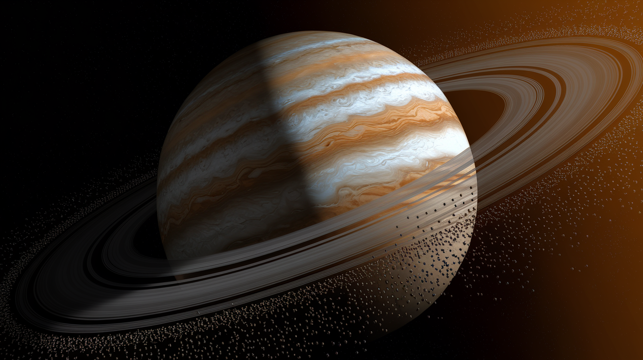
When a comet or asteroid kicks out debris, each dust grain inherits the parent body’s orbital elements at the moment of release. Fragmentation events create a cloud of particles with nearly identical a, e, i, ω, and Ω, differing only by small velocity kicks. Whether it’s a single nucleus breakup or continuous outgassing doesn’t change the basic picture. Over time this tight cluster disperses. Radiation pressure from sunlight pushes small grains outward, effectively lowering their perihelion distance or raising a slightly, depending on particle size. Larger meteoroids feel less push, so the stream develops a size-dependent spread in elements. Gravitational interactions with planets tug on the orbit, precessing Ω and ω at rates that depend on a, e, and i. The result is a ribbon of meteoroids stretched along the parent’s orbit, with element scatter that grows wider the older the stream.
Dispersion increases through radiation pressure, repeated fragmentation bursts, and secular evolution driven by planetary perturbations. Young streams stay narrow in Π and show tight radiant clustering. Old streams spread into broad filaments or even complete rings around the Sun. The CAMS dataset shows that a and e scatter more than q and i because speed measurement errors amplify uncertainties in semi-major axis and eccentricity. Still, the inherited pattern persists. Streams from Jupiter-family comets cluster at Tisserand parameter TJ around 2.0 to 2.5, while Mellish-type streams sit near TJ around 1.0 to 1.5, and asteroid-like Antapex sources push TJ above 3.0. Out-of-zone radiants can show TJ values of 4.3 to 9.6, flagging orbits shaped by strong planetary kicks or sungrazing encounters.
Using orbital-element clusters helps identify which debris filaments will intersect Earth at what time. A shower forecast starts with the parent body’s orbit, then applies backward integration to see when and where fragments were released. Forward integration from the breakup epoch reveals how Ω and Π evolved and predicts the solar longitude windows when filaments cross Earth’s path. Streams with nearly identical q, i, and Π but different Ω can produce separate peaks weeks apart, so splitting the stream by Π and node position is essential. The all-sky element maps show that Π separates showers temporally better than any other single parameter. That makes it the key to disentangling overlapping sources and pinning down exact peak timing.
Propagating Orbital Elements to Forecast Node-Crossing Dates

Observation-derived orbital elements are always tied to an epoch, the instant when position and velocity were measured. To forecast a future shower peak, you propagate those elements forward in time using the mean anomaly equation M(t) = M₀ + n(t – t₀), where mean motion n = √(GM☉/a³). At each forecast date, solve Kepler’s equation M = E – e sin E iteratively for eccentric anomaly, then convert to true anomaly f = 2 arctan[√((1+e)/(1–e)) tan(E/2)]. The particle crosses the ascending node when f + ω = 0° (mod 360°) and the descending node when f + ω = 180°. Compute the heliocentric distance r at that instant, then find Earth’s position from an ephemeris. The solar longitude of intersection is Ω (for ascending) or Ω ± 180° (for descending), adjusted by ω. Match that solar longitude to Earth’s calendar, and you have the predicted peak date.
Epoch choice matters because perturbations change Ω, ω, and even a and e over months to years. A set of elements valid in 2016 will drift by 2025, so re-fitting observations near the forecast year improves accuracy. Frame consistency is equally important. Barycentric elements (centered on the solar-system center of mass) differ slightly from heliocentric (Sun-centered) ones because the Sun wobbles around the barycenter. Long-term integrations show better stability in barycentric frames, but radiant calculations are simplest in heliocentric ecliptic coordinates. The CAMS computations use Sun-centered ecliptic longitude and latitude, with 20° solar-longitude windows advanced in 5° steps to track how element clusters shift over the year. That windowing technique directly illustrates how node positions evolve and helps identify which streams are active at which λ☉.
| Element | Influence on Node Timing |
|---|---|
| Ω | Directly sets the ecliptic longitude of the ascending node; shifts with precession, altering peak date by days per decade. |
| Π = ω + Ω | Combines node and perihelion orientation; strongest temporal clustering parameter; separates showers by peak solar longitude. |
| a | Controls orbital period and mean motion; large a means slow nodal precession and less frequent Earth encounters. |
| e | Affects radial velocity and time spent near perihelion; high e concentrates stream density near q, sharpening peak. |
| i | Determines radiant latitude and retrograde vs. prograde motion; influences nodal precession rate via secular terms. |
| M | Tracks particle position along orbit; solving Kepler’s equation for M at forecast date yields true anomaly and node-crossing time. |
Perturbations That Shift Meteor Shower Peak Timing
Gravitational tugs from Jupiter dominate long-term stream evolution, especially for orbits with semi-major axes near Jupiter’s 5.2 AU. The Tisserand parameter TJ ≈ 3 – (1/a + 2√(a(1 – e²)) cos i) is nearly conserved under Jupiter perturbations, so streams stay within characteristic TJ zones even as a and e fluctuate. Jupiter-family comet streams cluster at TJ around 2.0 to 2.5. Mellish-type orbits sit at TJ around 1.0 to 1.5. The retrograde Apex region includes particles with very low TJ, indicating long-period or near-parabolic origins. Over decades, close encounters with Jupiter can flip a stream’s node by several degrees, shifting the peak date by a week or more. Resonant interactions happen when the meteoroid’s orbital period is a simple ratio of Jupiter’s. They can lock Ω in place or cause it to librate, producing predictable timing variations or sudden jumps when the resonance breaks.
Non-gravitational forces add another layer. Poynting–Robertson drag removes orbital energy, slowly shrinking a and circularizing e, which shifts the node longitude inward over millennia. For millimeter-sized meteoroids, this effect is weak on human timescales but accumulates over tens of thousands of years, spreading old streams into broad arcs. The Yarkovsky effect (recoil from thermal emission) can push small grains sunward or outward depending on rotation, adding a size-dependent component to stream dispersion. Eccentricity-growth zones cluster near the transition regions at around 320° and 220° ecliptic longitude because those sky directions correspond to orbits where perturbations amplify e efficiently. Out-of-zone radiants with TJ values of 4 to 9 or higher flag particles that have experienced strong perturbation histories, sometimes including close solar passes that raised perihelion or resonant kicks that ejected them from the main stream.
Forecasting a peak requires modeling all these shifts. A simple two-body propagation assumes the Sun is the only mass, ignoring planets entirely. It works for a few months but drifts badly over years. Adding the eight planets in an N-body integrator captures secular precession and resonant effects. For high-precision outburst predictions (say, anticipating a dust trail from a comet’s 1950s perihelion passage), you also need to account for non-gravitational parameters fitted to the parent body’s motion. Each perturbation type modulates Ω, ω, and sometimes a or e, which together determine when and where Earth crosses the densest part of the stream.
Key perturbation types affecting shower timing:
Planetary gravity causes secular precession of Ω and ω, plus resonant locks or chaotic scattering.
Resonant interactions (mean-motion or secular resonances with Jupiter or Saturn) stabilize or destabilize node positions.
Thermal forces include Poynting–Robertson drag and the Yarkovsky effect shifting a and node longitude over long timescales.
Dissipative drag from solar radiation pressure on small grains effectively changes a and e and spreads the stream.
Techniques for Numerical Stream Forecasting

Numerical integration transforms a set of initial orbital elements into a future state by stepping through gravitational equations. For meteoroid streams, the workflow begins with a parent-body orbit and a release scenario, either a single burst or continuous ejection over several orbits. Each particle starts with elements slightly perturbed from the parent’s by an ejection velocity, typically a few meters per second. An N-body integrator like REBOUND or Mercury steps all particles forward in time, updating positions and velocities under the Sun’s gravity plus the eight planets. At each time step, you check whether a particle’s orbit crosses Earth’s. If it does, record the solar longitude and radiant coordinates. After running hundreds or thousands of virtual meteoroids, you bin the crossings by solar longitude and count how many land in each bin. The bin with the highest count marks the predicted peak.
The Öpik variables U, ϕ, and cos θ offer an alternative parameterization that feeds into dissimilarity criteria (D-criteria) for stream membership. U is the dimensionless speed (meteoroid velocity divided by Earth’s orbital speed). ϕ and cos θ encode the geometry of the encounter. These variables vary smoothly across the sky and correlate with classical elements, but on all-sky maps they don’t cleanly separate individual showers from the sporadic background. CAMS analysis shows that q, i, and ω form broad color zones larger than typical shower clusters, so small D-criterion thresholds are required to avoid lumping unrelated meteors together. MATLAB scripts and interactive plotting tools let you slide through 20° solar-longitude windows in 5° steps, watching element distributions shift and checking which streams are active when. Eccentricity peaks and semi-major-axis uncertainty both grow large for high-speed meteors, so N-body methods are essential when forecasting rare outbursts or modeling streams with e near 1.0.
Clone Ensemble Simulations
A single meteoroid orbit doesn’t capture the spread in ejection conditions or the measurement uncertainty in the parent body’s elements. Clone ensemble simulations address this by creating 100 to 10,000 virtual particles, each with slightly different a, e, i, ω, Ω, or release time, drawn from a covariance matrix or a Monte Carlo distribution. Every clone is integrated forward through the same planetary perturbations. As the ensemble evolves, you track the density of stream crossings along Earth’s orbit. Peaks in that density profile reveal when the stream is most concentrated. Secondary maxima hint at dust trails from specific perihelion passages of the parent comet. By binning crossing times into 0.001° solar-longitude intervals, you can resolve structure down to minutes. The ensemble spread also quantifies timing uncertainty. If 68% of clones cross within a ±0.01° window, the forecast has roughly that precision. This technique is the gold standard for predicting outbursts, because it maps the full range of possible arrival times given observational errors and model assumptions.
Error Sources and Forecast Uncertainty in Meteor Shower Timing
Speed measurement dominates uncertainty in a and e. A 1 km/s error in geocentric velocity can shift the computed semi-major axis by several AU for near-parabolic orbits, which translates to years of error in orbital period. Eccentricity is equally sensitive. A small speed error can flip e from 0.98 to 1.02, changing the orbit from a tight ellipse to a hyperbola. Even for well-observed meteors, video triangulation delivers speeds accurate to ±0.5 km/s at best, and radar Doppler sometimes does worse. That uncertainty propagates through the element computation and into the forecast. Southern-hemisphere coverage gaps compound the problem. CAMS v3.0 data stop at the end of 2016, leaving recent southern streams undersampled. Without fresh observations, you’re forecasting from old elements that may have drifted by a degree or more in Ω.
Sporadic contamination is another pitfall. The magnitude limit of around 5.5 for most optical networks means that faint showers blend into the background. Broad color zones in q, i, and ω maps show that those elements alone don’t isolate streams cleanly. You need small D-criterion thresholds to discriminate true members. Out-of-zone radiants can mimic shower orbits in single-element maps, producing false positives if you rely on just one parameter. Combining Π with temporal slicing (checking that meteors cluster in both Π and solar longitude) reduces these ghosts, but it requires a dense dataset and careful statistical tests. Covariance propagation or Monte Carlo stream simulations let you quantify how element uncertainties map to timing uncertainty, typically expressed as a ±1σ confidence interval in solar longitude or UTC hours.
Five key uncertainty drivers in meteor shower timing forecasts:
Velocity measurement error. Speed uncertainties of ±0.5 to 1 km/s propagate into large errors in a, e, and orbital period.
Epoch staleness. Using orbital elements from years-old data ignores secular precession and planetary perturbations that shift Ω and ω.
Incomplete sky coverage. Southern-hemisphere or daylight-radiant gaps leave some streams poorly constrained, increasing model variance.
Sporadic contamination. Broad element zones and magnitude limits blur the boundary between shower members and background, inflating false-match rates.
Perturbation model fidelity. Omitting non-gravitational forces or using simplified integrators introduces systematic drift in long-term forecasts.
Observational Validation and Calibration of Timing Predictions
Radar and video networks provide the ground truth for testing timing forecasts. The CAMS Meteoroid Orbit Database v3.0 relies on manual triangulation of video meteors, ensuring high-quality orbits down to visual magnitude around 5.5. Each detected meteor yields a radiant, speed, and orbital element set. Binning those meteors by solar longitude produces an observed activity profile. You compare the model’s predicted peak (solar longitude of maximum flux) against the empirical ZHR curve’s peak. If the model is off by more than ±0.02° in solar longitude (roughly ±30 minutes in time), you adjust the initial elements or tweak the perturbation parameters. Radar systems like CMOR detect fainter meteors and operate in daylight, filling gaps that optical cameras miss. Cross-checking radar radiants with video confirms that both see the same shower at the same time, building confidence in the element set.
The 72-frame solar-longitude windowing technique used in CAMS analysis directly validates the element-time mapping. By stepping through 5° increments in λ☉ and plotting orbital elements in each window, you watch clusters appear, peak, and fade. Streams with strong Π clustering show a tight correspondence between model-predicted λ☉ and observed activity. Weak or dispersed streams may have broader peaks or multiple subpeaks, flagging filamentary structure that a single-epoch element set misses. Historical shower records (decades of visual ZHR estimates, IMO data, and even older photographic orbits) extend the validation baseline. When a forecast matches archival peaks to within the observational scatter, you gain evidence that the perturbation model and element propagation are sound.
Calibration loops back into the forecast process. Discrepancies between predicted and observed peaks suggest either wrong initial elements or missing physics. Adding a non-gravitational parameter to the parent comet’s orbit, refining the ejection-velocity distribution, or switching to a higher-order integrator can all tighten the match. Each shower becomes a test case. Predict the 2025 Perseids using 2016 elements, observe the actual peak, then use the residual to update the model for 2026. Over multiple returns, systematic offsets shrink, and confidence intervals narrow. The result is a cycle where observations feed models, models generate forecasts, and new observations validate or correct those forecasts.
Four data types used to validate timing forecasts:
Video meteor orbits deliver high-precision radiant, speed, and element sets for meteors brighter than around mag 5.5. Manual triangulation ensures quality.
Radar detections offer continuous monitoring, daylight capability, and fainter magnitude reach. Doppler velocities confirm vg and orbital speed.
Visual ZHR curves from observer networks give hourly zenithal rates. Peak timing to ±0.1° solar longitude when well-sampled.
Historical records include decades of archived activity profiles, photographic orbits, and early radar campaigns. They anchor long-term trend analysis.
Final Words
We turned orbital elements into calendar dates: perihelion distance q and perihelion longitude Π map to radiants, and the node Ω marks the crossing. We showed how propagation, perturbations, and clone integrations pick the peak windows.
We also covered error sources and how radar, video, and historical records refine forecasts. It’s a mix of dynamics and careful observation, doable with standard ephemerides and tools.
This guide to using orbital elements to forecast meteor shower timing ties the mechanism to practical steps, so you can predict and confirm peaks. Worth the effort, clear skies ahead.
FAQ
Q: How do the six orbital elements tell us when Earth will meet a meteoroid stream?
A: The six orbital elements tell us timing by locating where the stream’s orbit crosses Earth’s path and when stream particles reach that node, using q = a(1–e) and the orbit angles to set the encounter moment.
Q: Why are Ω (longitude of ascending node) and Π = ω + Ω the best predictors of peak solar longitude?
A: Ω and Π are best predictors because Ω fixes the node’s ecliptic longitude and Π = ω + Ω groups perihelion timing, so Π gives the strongest temporal clustering that separates showers by date.
Q: How do we convert nodal longitudes to calendar dates using ephemerides like JPL Horizons?
A: You convert nodal longitudes to dates by using an ephemeris to get Earth’s heliocentric ecliptic longitude, matching that solar longitude to the node, then translating the solar longitude into a UTC calendar date.
Q: What are the practical steps from orbital elements to a predicted UTC peak date?
A: The practical steps are: compute true anomaly at the node from element set, find stream position at that anomaly, calculate solar longitude of intersection, convert solar longitude to UTC via ephemerides, confirm with radiant prediction.
Q: How do a, e, and i influence stream timing and radiant motion?
A: a, e, and i influence timing because a sets orbital period, e changes perihelion timing and q, and i alters the encounter geometry and radiant drift, so their combination shifts when Earth meets dense stream parts.
Q: What are mean, eccentric, and true anomaly and why does true anomaly at node determine intersection timing?
A: Mean, eccentric, and true anomaly are different measures of position along an orbit; true anomaly gives the actual location at a given time, so true anomaly at the node directly fixes when the stream crosses Earth’s path.
Q: How does a parent body’s orbit map to a meteoroid stream and affect peak timing?
A: A parent body’s orbit maps to a stream because released debris shares the parent’s elements; dispersion from radiation pressure, fragmentation, and secular forces spreads the stream while Π, q, and T_J keep timing signatures.
Q: Why do perturbations shift predicted peak dates and which forces matter most?
A: Perturbations shift peak dates because planetary gravity, resonances, and thermal forces change a, e, and node locations; Jupiter perturbations, resonance sweeping, and Poynting–Robertson drag are especially important.
Q: What numerical methods are used to forecast stream peaks and why use clone ensembles?
A: Forecasting uses N-body integrators like REBOUND to forward-integrate particles; clone ensembles of 100–10,000 particles map density maxima along the stream and reveal likely peak dates despite dispersion and uncertainties.
Q: What are the main error sources in timing forecasts and how are uncertainties estimated?
A: Main error sources are speed uncertainties that skew a and e, epoch/frame mismatches, catalog gaps, and sporadic contamination; Monte Carlo clone simulations propagate those errors into confidence intervals for peak dates.
Q: How do observations validate and refine predicted peak dates?
A: Observations validate and refine dates by comparing radar, video, and visual ZHR curves to model solar-longitude windows, then adjusting element sets or integration parameters to improve timing agreement.