
What if your telescope can’t tell two nearby colors apart?
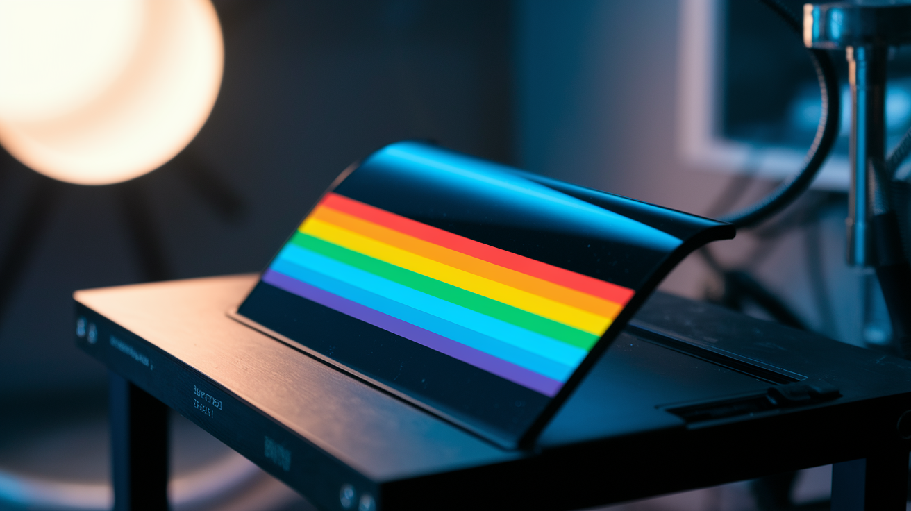
That’s spectral resolution in action: a number that says how sharply a spectrograph splits adjacent wavelengths.
Higher resolution pulls apart crowded spectral lines, finds tiny Doppler shifts, and lets astronomers read chemical fingerprints (like a barcode of light).
Lower resolution blends features but gives more signal.
This post shows what spectral resolution measures, why it matters for velocity and abundance work, and which instrument choices and limits decide what you can actually see.
Core Meaning of Spectral Resolution for Telescope Observations
Spectral resolution measures how well a telescope’s spectrograph can split apart wavelengths that sit close together. It’s basically the instrument’s sharpness when looking at neighboring colors in a spectrum. Two emission or absorption lines bunched together in wavelength will appear as separate features in a high-resolution system. A low-resolution setup smears them into one broad hump.
You’ll see the metric reported two ways. First is Δλ, the smallest wavelength gap the instrument can cleanly resolve, usually in nanometers (nm) or Angstroms (Å). One Angstrom equals 0.1 nanometer. Second is resolving power, written R = λ / Δλ, where λ is the wavelength you’re studying. R has no units. Higher numbers mean finer detail. Say your spectrograph measures Δλ = 0.11 nm at λ = 500 nm. Then R comes out around 4,545. Drop to Δλ = 2.44 nm at the same wavelength and R falls to roughly 205.
Astronomers lump instruments into rough categories. Low resolving power runs from about R = 100 to 1,000, where you catch coarse features and blended lines. Medium resolution lives around a few thousand. High resolution kicks in near R = 20,000 and stretches past 100,000, enough to separate tightly packed lines and track tiny wavelength shifts. Velocity precision scales straight with R through Δv ≈ c / R, where c is the speed of light at roughly 3.0 × 10⁵ km/s. At R = 20,000 you land around 15 km/s velocity precision. Push to R = 100,000 and you hit roughly 3 km/s.
The real-world impact for telescope work breaks into four areas:
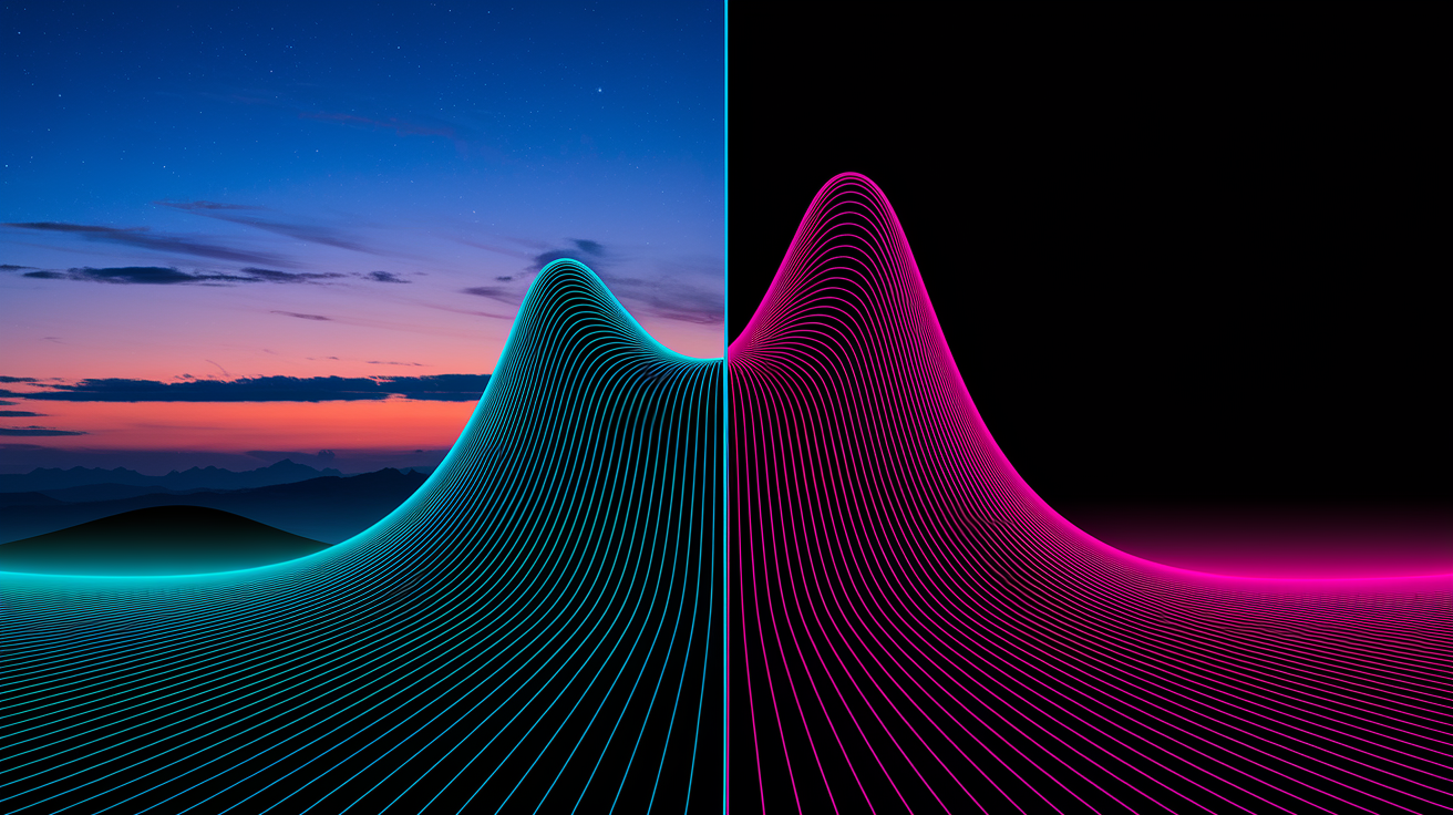
Line blending: Low resolution mushes adjacent lines together. High resolution pulls them apart for separate measurement.
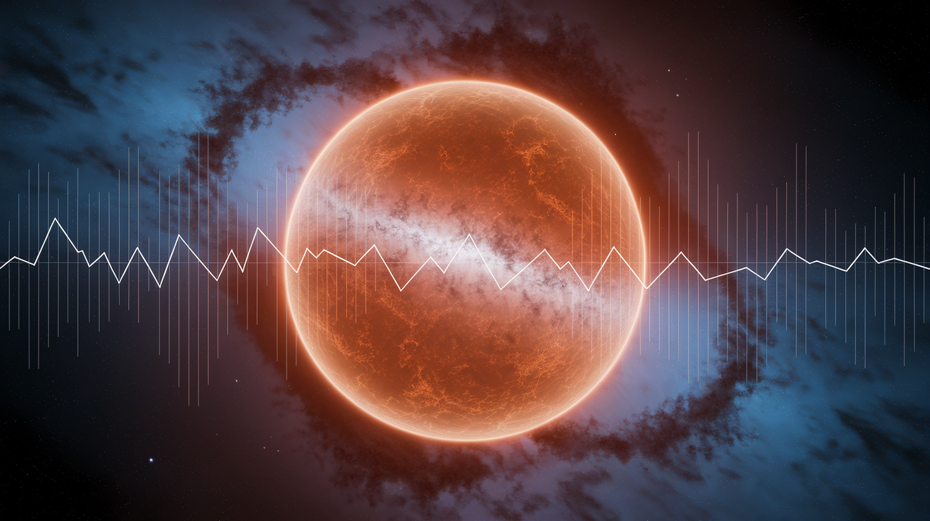
Velocity and redshift accuracy: Finer Δλ lets you measure smaller Doppler shifts, which matters for exoplanet hunting, galaxy motion studies, and cosmological redshifts.
Chemical abundance detail: Resolving weak, closely spaced lines reveals trace elements and isotope ratios in stellar atmospheres and nebulae.
Physical diagnostics: Line width and profile shape carry information about temperature, density, turbulence, and magnetic fields. You need decent resolution to see those details.
How Telescope Spectrographs Generate and Limit Spectral Resolution
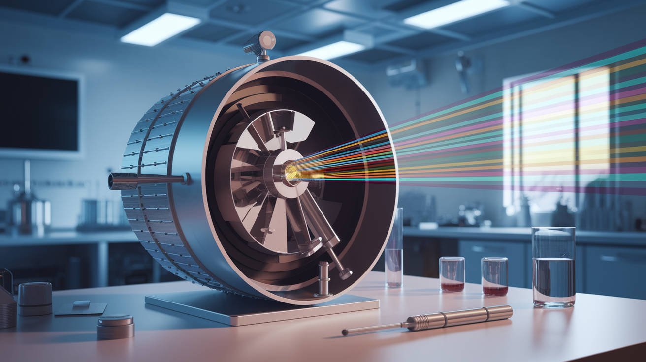
A spectrograph funnels incoming light through a narrow entrance slit, straightens it with mirrors or lenses, sends it through something that spreads wavelengths into a spatial rainbow, then focuses that rainbow onto a detector. Every step shapes the final spectral resolution. The entrance slit width sets how much of the light beam you’re starting with. Narrower slits give you sharper spectral lines but let in less total light. A 10-micron slit might deliver crisp lines, while a 100-micron slit boosts your signal but broadens every feature. You’re balancing throughput against sharpness, and that trade-off forces choices between sensitivity and clarity.
Optical quality counts too. The system’s Point Spread Function, shaped by diffraction, aberrations, and atmospheric seeing (for ground telescopes), sets a floor on how sharp your spectrum can be. If the PSF stretches 20 microns wide, closing the slit below that width buys you almost nothing because diffraction and imaging blur take over. Resolution doesn’t improve forever as you tighten the slit. There’s a sweet spot, usually where slit width matches the PSF size, giving you the best spectral sharpness without throwing away photons.
Dispersive Elements and Detector Sampling
The dispersive element (most often a diffraction grating) controls how much the spectrum spreads across the detector. Gratings are ruled with closely spaced grooves, typically 150 to 3,000 lines per millimeter. Higher groove density boosts angular dispersion, spreading the spectrum wider and shrinking Δλ for a given detector size. A Kymera 193i spectrograph with a 150 line/mm grating measured Δλ = 2.44 nm, while a Shamrock 750 with a 600 line/mm grating reached Δλ = 0.11 nm under similar conditions. Prisms also spread light but rely on how refractive index changes with wavelength, producing less dispersion and lower resolving power than high-density gratings for the same physical footprint.
Detector pixel size sets the sampling limit. A spectrum gets recorded by an array of pixels, each one collecting light over its width. Large pixels (say 50 microns) chop fine spectral detail into coarse bins, and you lose resolving power even if the optics and grating deliver better. Smaller pixels, around 10 to 15 microns, sample the spectrum finely and keep the resolution the rest of the system provides. There’s a Nyquist rule: you need at least two pixels per resolution element to avoid undersampling and information loss.
| Factor | Effect on Δλ |
|---|---|
| Slit width | Narrower slit → smaller Δλ (until PSF limit); wider slit → larger Δλ, more light |
| Grating line density | More lines/mm → greater dispersion → smaller Δλ at detector |
| Detector pixel size | Smaller pixels → finer sampling → preservation of native Δλ; larger pixels → quantization → effective Δλ increase |
Quantitative Examples Showing What Different Levels of Spectral Resolution Reveal
Numbers make this concrete. At λ = 500 nm, an instrument with Δλ = 2.44 nm gives you R ≈ 205. That’s low resolution. Spectral features broader than a few nanometers merge, and you mostly see continuum slope and very broad absorption or emission humps. Switch to Δλ = 0.11 nm and R jumps to roughly 4,545. Now you start resolving individual strong lines, separating doublets that sit a few tenths of a nanometer apart, and measuring line centers with useful precision.
Velocity resolution follows straight from that. Using Δv ≈ c / R with c = 3.0 × 10⁵ km/s, an R = 2,000 instrument gives you Δv around 150 km/s. That’s enough to tell a galaxy’s systemic redshift from zero but not enough to trace internal rotation or measure stellar speeds better than a few hundred km/s. Push to R = 20,000 and Δv drops to about 15 km/s, good for most stellar velocity work. At R = 100,000, Δv falls near 3 km/s, the territory where you hunt for tiny exoplanet wobbles or resolve turbulence in stellar atmospheres.
Line blending shows another clear split. Picture two absorption lines separated by 0.3 nm. At R = 1,000 (Δλ ≈ 0.5 nm at 500 nm) the lines merge into one broad dip. At R = 5,000 (Δλ ≈ 0.1 nm) you see a saddle or slight valley between them. At R = 20,000 (Δλ ≈ 0.025 nm) both lines stand cleanly apart, each with its own depth, width, and central wavelength. That separation matters for chemical abundance work. If you can’t isolate a weak line from its neighbor, you can’t measure its strength or figure out the element’s abundance.
Here’s what changes across resolution regimes:
- Line width appearance: Low R makes all lines look like broad smears. Medium R reveals approximate profiles. High R captures true line shapes and fine structure.
- Blending and confusion: At low R, multiplets and close doublets collapse into single features. High R separates them for individual analysis.
- Velocity accuracy: Low R limits you to redshift surveys and rough motion studies. Medium R handles basic radial velocity measurements. High R reaches precision velocity work for dynamics and exoplanet detection.
- Abundance sensitivity: Weak lines and isotopic shifts vanish in low-R data. High R makes them visible and measurable, opening detailed chemical mapping.
High-Resolution Spectroscopy and Its Telescopic Science Applications
High spectral resolution (typically R above 20,000, often 50,000 to 100,000 or more) unlocks science you can’t do any other way. The narrow line widths and precise wavelength measurements let you separate blended features, resolve fine structure, and detect small velocity shifts that carry critical physical information. Stellar abundance studies depend on it. A Sun-like star’s spectrum holds thousands of absorption lines, many packed close together. To measure the strength of a weak iron line sitting 0.05 nm from a stronger titanium line, you need R well above 10,000. Stretch that to rare-earth elements or isotopic ratios and R = 50,000 becomes the baseline.
Nebular diagnostics also demand high resolution. Emission-line regions in planetary nebulae, H II regions, and active galactic nucleus outflows produce narrow lines (sometimes only a few km/s wide intrinsically) and closely spaced forbidden-line doublets. Resolving those doublets (often separated by less than 1 nm) and measuring their relative intensities reveals electron density and temperature. Low-R spectra blend the lines and you lose that diagnostic power.
Exoplanet and Stellar Velocity Measurements
Detecting exoplanets through the radial velocity method means measuring Doppler shifts smaller than the orbital speed the planet causes. A Jupiter-mass planet on a one-year orbit around a Sun-like star pulls the star at roughly 12 m/s. Converting that to wavelength shift at 500 nm gives Δλ ≈ 0.00002 nm. You can’t directly resolve that, but you can measure it by cross-correlating thousands of spectral lines, each shifted by that tiny amount. The trick is having enough resolution so the lines themselves are narrow and well sampled. Typical exoplanet spectrographs run R = 70,000 to 120,000. Below about R = 50,000, line blending and broad profiles mess up the cross-correlation signal and push velocity uncertainties past the few m/s precision you need.
Stellar rotation and atmospheric turbulence show up in line profiles too. A rotating star Doppler-broadens its absorption lines. Measuring that broadening to get v sin i (projected rotational velocity) needs R high enough that the instrumental profile doesn’t drown the real width. For slow rotators (v sin i < 10 km/s) you want R above 30,000. Fast rotators are easier, but if you want to resolve asymmetries or catch differential rotation, R = 50,000 or more helps.
Chemical Abundances and Nebular Diagnostics
Abundance analysis relies on measuring equivalent widths (the integrated depth of an absorption line) and comparing observed line strengths to synthetic spectrum models. Weak lines give the most reliable abundances because they’re not saturated, but weak lines also blend easily with neighbors or get lost in noise. High resolution separates them. The rare-earth element europium has several lines in the blue-green that sit within 0.2 nm of iron and chromium lines. At R = 10,000 they overlap. At R = 40,000 they stand apart.
Nebular forbidden lines often form doublets from fine-structure splitting. The [O III] λ4959, λ5007 Å pair is well separated (roughly 5 nm), but others like [S II] λ6716, λ6731 Å sit only 1.5 nm apart. The intensity ratio of that doublet is density sensitive. Measure it and you figure out the nebula’s electron density. At R = 3,000 (Δλ ≈ 2 nm at 670 nm) the lines blur together. At R = 10,000 (Δλ ≈ 0.67 nm) you see two peaks but the wings overlap. At R = 20,000 or higher they separate cleanly and photometry becomes straightforward.
Low and Medium Spectral Resolution for Surveys and Broadband Studies
Not every science goal needs high resolution. Plenty of astronomical programs deliberately choose low or medium R to gain sensitivity, speed, or spatial coverage. Low-resolution spectroscopy (R from 100 to roughly 1,000) captures the continuum shape, broad absorption or emission features, and overall color gradient. That’s enough to classify galaxies by type, measure approximate redshifts from broad lines, or identify a star’s spectral class. Survey instruments often use R ≈ 200 to 500 to maximize the number of objects observed per night, trading spectral detail for photon-gathering power and wide-field multiplexing.
Medium resolution, around R = 2,000 to 5,000, strikes a balance. You resolve most individual strong lines, can measure rough radial velocities (to a few tens of km/s), and identify the main chemical features without the cost and complexity of high-R systems. Medium-R spectra are common in galaxy redshift surveys, stellar parameter pipelines, and follow-up spectroscopy of transient sources where you want quick classification rather than detailed abundance analysis. The broader Δλ boosts per-channel signal to noise because more photons land in each wavelength bin, and shorter exposures work for faint targets.
The choice depends on your question:
Low R (100 to 1,000): Use for redshift surveys, continuum slope measurements, broad feature identification, and high-throughput multi-object spectroscopy. Exposure times are short and faint objects become reachable.
Medium R (2,000 to 5,000): Pick for stellar classification, approximate abundances, modest velocity precision, and follow-up of transients or variables. You get enough detail to separate major lines without the instrumental cost and long integrations of high R.
High R (> 20,000): Reserve for precision velocity work, detailed chemical analysis, line profile studies, and any science needing narrow-line separation or sub km/s velocity accuracy. Exposure times grow and SNR per resolution element drops, so targets must be bright or telescope aperture large.
Calibration, Stability, and Sampling Requirements That Preserve Spectral Resolution

Getting the spectrograph’s advertised spectral resolution on sky takes careful wavelength calibration and instrumental stability. Calibration lamps (historically hollow-cathode lamps filled with thorium-argon gas) provide emission lines at known wavelengths. You record a calibration exposure, identify the lines, and build a wavelength solution mapping pixel number to λ. ThAr works well for medium to high R but has limits. Line density is uneven across the spectrum, some spectral regions lack strong lines, and the lamp spectrum can drift slightly over time from pressure or temperature changes. Modern high-precision work increasingly uses laser frequency combs, which produce thousands of evenly spaced lines with wavelength accuracy better than 1 m/s equivalent, ideal for exoplanet radial velocity programs.
Instrumental broadening (the spectrograph’s own contribution to line width) must be measured and, when possible, removed. Every system blurs incoming light through the slit profile, optical aberrations, and pixel integration. You characterize this by observing a narrow-line calibration source or unresolved emission line and fitting the resulting line shape. That measured profile (often called the instrumental Line Spread Function or LSF) can then be deconvolved from science spectra to recover true line shapes. Skip this step and measured line widths always come out larger than the real astrophysical values, biasing velocity and temperature measurements.
Sampling matters as much as raw resolution. The Nyquist theorem says you need at least two detector pixels per resolution element to capture all the information the optics deliver. Undersample (one pixel per resolution element or worse) and you lose spectral detail and introduce aliasing. Oversample to three or four pixels per element and you get cleaner line profiles and easier interpolation, at the cost of more read noise and larger data files. Most modern échelle and long-slit spectrographs aim for roughly 2.5 to 3.5 pixels per resolution element as a practical sweet spot.
| Type | Precision Level | Limitations |
|---|---|---|
| ThAr hollow-cathode lamp | ~10 to 50 m/s wavelength accuracy | Uneven line coverage; long-term pressure and temperature drift; needs regular re-calibration |
| Laser frequency comb | ~1 m/s or better | Expensive; complex setup; not yet standard on all telescopes |
| Iodine absorption cell | ~3 to 10 m/s (for radial velocity) | Limited to specific wavelength range (500 to 620 nm); complicates data reduction; line blending with stellar spectrum |
Thermal and mechanical stability keep the wavelength solution steady between calibrations. Temperature swings shift grating angles and detector positions, drifting line centers across pixels. High-stability instruments use temperature control (often to millikelvin precision) and rigid optical benches. Fiber-fed spectrographs isolate the disperser in a vacuum chamber to kill air pressure wavelength shifts. Stability also applies to the detector. Read noise, dark current, and cosmic ray hits add noise that cuts effective spectral resolution when SNR is low. Cooling the CCD reduces dark current, and careful readout modes minimize electronic noise.
Choosing the Right Spectral Resolution for Telescope Observing Programs

Picking spectral resolution is a multi-way trade. Higher R gives you finer wavelength detail but costs light, time, and sometimes spatial coverage. First step is matching your science question to the minimum required resolving power. If you’re measuring a galaxy’s systemic redshift from [O II] λ3727 Å emission, R = 500 is plenty. The line is intrinsically broad and you only need the centroid. Searching for a 5 m/s exoplanet signal? You need R above 70,000 and rock-solid stability. Write down the velocity precision or line separation requirement, convert it to Δλ or R, then add margin for real-world conditions like blending and continuum noise.
Next, check your target brightness and available telescope time. Exposure time calculators (most observatories provide them) take your target magnitude, desired SNR, and chosen R as inputs and spit out the required integration time. You’ll often find that doubling R quadruples exposure time, because higher dispersion spreads the same photons over more pixels and narrower slits let in less light. If the calculator says six hours for one star at R = 100,000 but only 45 minutes at R = 30,000, ask whether your science truly needs the higher resolution. Sometimes it does. Often a compromise resolution still answers the question and lets you observe more targets or go deeper in magnitude.
Practical setup tips that keep resolution intact and avoid wasted effort:
Match slit width to atmospheric seeing: On a ground-based telescope, if seeing is 1.2 arcsec and your slit is 0.5 arcsec, you lose light and gain little resolution because the star image is bigger than the slit. A 1.0 to 1.5 arcsec slit captures more flux and still delivers the resolution set by the PSF, not the slit.
Check detector pixel scale against required sampling: Confirm that the spectrograph’s native dispersion gives at least 2 pixels per resolution element. If not, you’re paying for high R on paper but throwing away the detail in undersampled data.
Balance SNR and resolution: For weak lines, SNR often matters more than ultra-high R. A spectrum at R = 40,000 with SNR = 100 will give better abundance precision than R = 100,000 with SNR = 30, because measurement uncertainty scales with noise.
Use calibration data and stability checks: Grab calibration frames before and after science exposures. Monitor wavelength solution drift. If your lamp lines shift by half a pixel during the night, your actual resolution and velocity accuracy degrade no matter what the spectrograph spec sheet says.
Final Words
We defined spectral resolution as the ability to separate closely spaced wavelengths, showed Δλ and R = λ/Δλ, and gave hands-on examples that tie numbers to velocity precision.
Then we traced how slits, gratings, detector pixels, and calibration set real limits, and why low, medium, and high R suit different surveys and science goals like exoplanet velocities or abundance work.
Understanding spectral resolution what it means for telescopes helps you pick the right instrument and exposure. Go look at a spectrum. You’ll see how those numbers matter.
FAQ
Q: What is meant by spectral resolution?
A: Spectral resolution means the ability to separate closely spaced wavelengths. It’s measured as Δλ (smallest distinguishable wavelength, in nm or Å) or as resolving power R = λ/Δλ, with higher R separating finer features.
Q: What does 30m spatial resolution mean?
A: A 30 m spatial resolution means each image pixel covers about 30 meters on the ground, so details smaller than 30 meters will blur together; it describes the smallest distinguishable feature size in the image.
Q: Why is spectral resolution important?
A: Spectral resolution is important because it separates blended spectral lines, enables accurate chemical identification and redshift or Doppler velocity measurements, and sets how precisely you can measure motions or abundances.
Q: What is an example of spectral resolution?
A: An example of spectral resolution: at 500 nm, Δλ = 2.44 nm gives R ≈ 205 (low R), while Δλ = 0.11 nm gives R ≈ 4,545 (higher R), showing smaller Δλ yields greater resolving power.