
Can satellites tell when a forest is truly gone, or just hiding behind clouds?
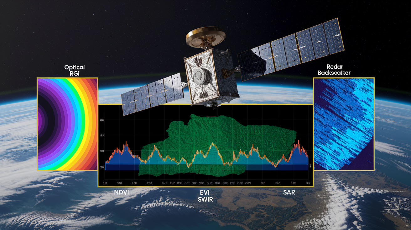
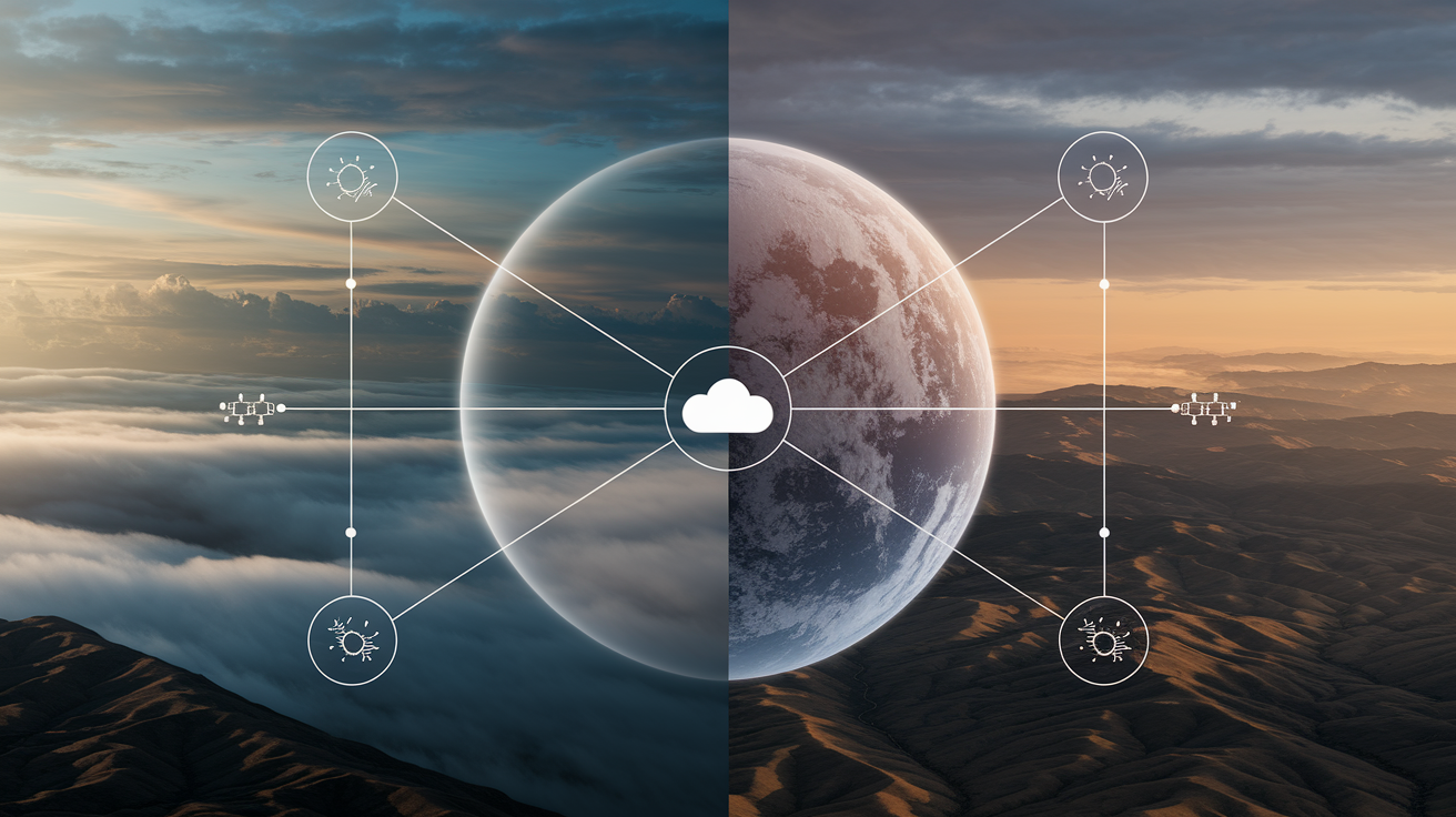
Satellites read a site’s “light fingerprint”, how visible, near-infrared, and shortwave-infrared light bounce back, and also listen with radar (radio pulses that map structure).
By spotting sudden drops in greenness indices like NDVI (a simple measure of plant vigor), matching them to weaker radar backscatter, and checking decades of archive photos, analysts separate real, permanent clearing from seasonal or temporary changes.
The result: faster, more reliable alerts that help stop illegal clearing sooner.
Core Principles Behind Detecting Forest Loss from Satellite Imagery
Satellites keep recording Earth’s surface in multiple wavelengths: visible light, near-infrared, shortwave infrared, radar. Healthy forests absorb most red light but bounce back a ton of near-infrared, thanks to chlorophyll and the way leaves are built. Cut down the canopy and the whole signature flips. Exposed soil or cleared ground throws back more red and shortwave infrared, way less near-infrared. The shift happens fast. A satellite passes over fresh clearing and registers a sudden change in the light fingerprint, visible even from hundreds of kilometers up.
But optical data alone? Misleading. Clouds, seasonal leaf drop, temporary logging roads can all look like permanent clearing when they’re not. That’s why analysts stack optical vegetation indices like NDVI (Normalized Difference Vegetation Index) and EVI with radar backscatter changes. Radar sends a pulse of radio waves toward the forest, measures how much energy comes back. Intact canopy scatters the signal everywhere, strong return. Bare ground or short vegetation reflects much less. When both the optical greenness drops and the radar backscatter weakens at the same spot, confidence goes up that the forest’s actually gone, not just hidden or dormant for the season.
Historical archives and frequent revisits separate fleeting disturbances from permanent deforestation. Landsat’s been recording Earth since 1984. Analysts check whether a flagged area was forested decades ago and stayed that way until the new clearing appeared. Sentinel-2’s five-day revisit and MODIS daily coverage catch events soon after they happen. Stack images over weeks or months and algorithms can tell the difference between a one-time harvest, a fire scar that regrows, a seasonal crop cycle, or a forest permanently turned into pasture.
Core physical signals that reveal deforestation:
NDVI drop – sudden decline in the normalized difference between near-infrared and red reflectance, showing loss of photosynthetically active vegetation.
SWIR increase – shortwave infrared reflectance jumps when dry soil or dead biomass replaces moist canopy.
Bare-soil reflectance rise – cleared areas expose mineral soil with bright visible and shortwave signatures.
SAR backscatter reduction – radar return weakens when vertical canopy structure disappears, replaced by flat, low-roughness surfaces.
Thermal anomaly from fires – infrared sensors pick up heat spikes during active burning, tagging deforestation driven by slash-and-burn clearing.
Optical Satellite Sensors and Spectral Indicators Used in Forest Loss Detection

Healthy vegetation soaks up most incoming red light for photosynthesis, reflects nearly half of the near-infrared that hits leaves. Strong contrast. Cut the forest and the ground reflects more red (no chlorophyll absorbing it) and less near-infrared (leaf structure’s gone). Shortwave infrared bands are especially touchy about moisture and structural changes. Cleared land with dry litter or exposed soil shows a sharp jump in SWIR reflectance. Compare before and after brightness in these bands and algorithms calculate indices like NDVI or Enhanced Vegetation Index, which both drop hard when canopy disappears.
Analysts set thresholds based on seasonal baselines to dodge false positives. Deciduous forests naturally lose leaves each autumn, temporary NDVI dip. The algorithm learns this annual cycle from multi-year data and ignores regular seasonal swings. Burn scars show distinct spectral patterns: high SWIR reflectance combined with low near-infrared, often a lingering char signature. So a Normalized Burn Ratio (NBR) can tell fire-driven clearing from mechanical logging. Sentinel-2’s 10 to 20 meter resolution captures these patterns across large areas every few days, Landsat’s 30-meter archive extends the record back four decades, and MODIS at 250 to 500 meters provides daily snapshots useful for spotting large, fast events even if fine detail is lost.
| Index/Band | Role | Sensitivity Notes |
|---|---|---|
| NDVI (NIR − Red)/(NIR + Red) | Quantifies greenness and photosynthetic activity | Drops sharply when canopy is removed; can saturate in very dense forests |
| SWIR (1.5–2.5 µm bands) | Detects moisture content and soil/litter exposure | Rises when dry biomass or bare soil replaces moist leaves; key for separating logging from phenology |
| NBR (NIR − SWIR)/(NIR + SWIR) | Highlights burn scars and fire-affected areas | Negative change (pre-fire minus post-fire NBR) isolates burned patches from other disturbances |
Radar and SAR Backscatter Signals for Cloud‑Free Deforestation Monitoring
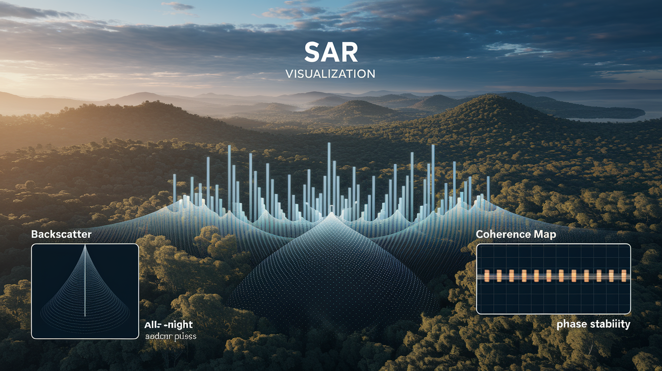
Synthetic Aperture Radar sensors send pulses of radio waves toward the surface, measure the strength of the echo. Forest canopies, with their vertical trunks, branches, layered leaves, scatter radar energy in many directions. Some bounces back to the satellite, producing a strong return signal. Cleared ground is much flatter and simpler. Less energy scatters back. The backscatter coefficient drops noticeably when trees are removed. Radar uses its own illumination rather than sunlight, so it works equally well day or night and penetrates clouds, rain, smoke that would block optical sensors. Indispensable in tropical regions where persistent cloud cover hides deforestation for weeks in optical imagery.
Coherence-based methods add another layer. Interferometric SAR compares the phase of radar returns from two passes over the same area. Stable surfaces like intact forest or bare rock maintain high coherence between images. Changes in canopy structure (branches moved, trees cut) destroy the phase relationship and coherence drops. Multi-temporal SAR stacks track both backscatter and coherence over dozens of dates, revealing even subtle canopy degradation from selective logging or gradual thinning that optical indices might miss. Sentinel-1 provides roughly 10-meter resolution with a 6 to 12 day revisit, continuous monitoring in regions where optical satellites see only scattered cloud-free glimpses.
SAR advantages for deforestation monitoring:
Cloud and weather independence – radar signals penetrate clouds, rain, haze, smoke without degradation.
Day and night operation – no sunlight required. Imaging happens on any orbit, doubling potential observation frequency.
Sensitivity to vertical structure – backscatter responds to canopy height and density, effective for detecting partial canopy removal.
Complementary to optical data – fusing SAR with NDVI/EVI outputs reduces false positives and fills temporal gaps, improving detection confidence and timeliness.
Key Satellite Programs Used to Monitor Forest Change Globally
Landsat satellites have mapped Earth at roughly 30-meter resolution since 1984. Longest continuous archive of moderate-resolution imagery available. The 16-day revisit interval means each location gets observed about twice a month under clear skies, and the historical depth lets analysts confirm that a patch of forest existed for decades before it was cleared. Landsat’s archive underpins long-term trend studies and provides the baseline against which new losses are measured. Sentinel-2, operated by the European Space Agency, carries a similar multispectral sensor but flies as a two-satellite constellation with 10 to 20 meter resolution and a combined revisit of roughly five days. Higher temporal frequency catches clearing events sooner and improves the odds of capturing cloud-free images in humid tropics.
MODIS instruments aboard NASA’s Terra and Aqua satellites offer daily global coverage at 250 to 1,000 meter resolution depending on the spectral band. Too coarse to map small clearings or narrow logging roads, but MODIS excels at detecting large-scale forest loss, tracking active fires in near real-time, monitoring seasonal vegetation trends across entire countries. Commercial constellations like Planet’s PlanetScope provide 3 to 5 meter resolution with near-daily revisits. High-resolution SAR satellites deliver meter-scale imagery on demand. These come at higher cost and require tasking or subscription access, but they catch early detection of road building, small plantation expansions, other changes invisible to moderate-resolution sensors.
| Satellite | Resolution | Revisit | Primary Use |
|---|---|---|---|
| Landsat 5/7/8 | ~30 m (multispectral) | 16 days | Long-term archive; trend analysis; baseline mapping back to 1984 |
| Sentinel-2A/2B | 10–20 m (key bands at 10 m) | ~5 days (constellation) | Frequent optical monitoring; higher spatial detail than MODIS; operational change detection |
| MODIS (Terra/Aqua) | 250–500 m (visible/NIR) | Daily | Broad-scale trends; fire detection; rapid event detection over large areas |
| Sentinel-1A/1B (SAR) | ~10 m (IW mode) | 6–12 days (area-dependent) | All-weather monitoring; cloud-penetrating change detection; tropical forest tracking |
Resolution and revisit frequency trade against coverage and cost. High-resolution commercial sensors see individual trees and narrow roads but cover smaller footprints per pass and often require payment. Landsat and Sentinel data are free and global but miss the finest details. Programs monitoring vast tropical estates often layer multiple sensors: MODIS for rapid alerts, Sentinel-2 for routine mapping, and tasked high-resolution optical or SAR to investigate priority hotspots.
Change Detection Algorithms for Identifying Deforestation
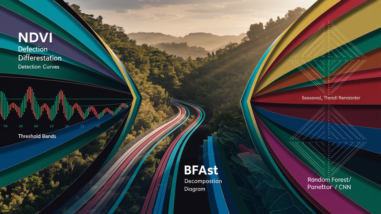
Image differencing is the simplest approach. Subtract a baseline image from a recent acquisition, and pixels that changed dramatically stand out. Analysts often difference vegetation indices rather than raw bands. Subtracting today’s NDVI from last year’s NDVI highlights areas where greenness dropped. Thresholding converts the difference into a binary forest-loss map by flagging any pixel that fell below a defined NDVI threshold. Works well for abrupt clearcuts but struggles with gradual degradation or seasonal variation. More sophisticated methods stack many dates into a time series and search for structural breaks.
BFAST (Breaks For Additive Season and Trend) decomposes a time series of NDVI or other indices into seasonal, trend, and remainder components, then detects abrupt changes in the trend that exceed normal seasonal swings. CCDC (Continuous Change Detection and Classification) fits harmonic models to each pixel’s history and flags the date when observations no longer match the expected seasonal pattern, producing a continuous monitoring stream rather than periodic snapshots. Both reduce false positives caused by phenology, clouds, or temporary disturbances because they learn what “normal” variation looks like from years of data.
Machine learning classifiers (Random Forest, Support Vector Machines, convolutional neural networks) train on labeled examples of forest, cleared land, and intermediate states, then predict the class of every pixel in a new image. Object-based image analysis segments the scene into meaningful patches (forest stands, fields, roads) before classifying, capturing spatial context that per-pixel methods miss. Deep learning models learn complex patterns directly from stacked multi-date, multi-sensor inputs, automating feature extraction and improving accuracy when training data are plentiful. These ML approaches often fuse optical indices, SAR backscatter, terrain data, and auxiliary layers into a single prediction, using all available information to distinguish true deforestation from look-alikes.
Commonly used change-detection algorithms:
Image differencing and thresholding – fast, simple. Effective for clear-cut events but sensitive to clouds and seasonality.
BFAST (Breaks For Additive Season and Trend) – decomposes time series to isolate abrupt trend breaks from seasonal cycles.
CCDC (Continuous Change Detection and Classification) – harmonic modeling of pixel history. Flags departures from expected pattern in near real-time.
Supervised machine learning (Random Forest, SVM) – trains on labeled samples to classify forest vs. non-forest and predict change probability.
Deep learning (CNNs, U-Net architectures) – learns spatial and temporal features from multi-sensor stacks. High accuracy when training data and compute are available.
Preprocessing and Data Cleaning Required Before Detecting Forest Loss
Raw satellite data arrive as digital numbers that need correction for geometric distortions, atmospheric scattering, sensor calibration drift before they can be compared across dates. Orthorectification removes terrain-induced shifts so that pixels align precisely with ground coordinates, essential when stacking images from different orbits or sensors. Atmospheric correction converts top-of-atmosphere radiance into surface reflectance by estimating and subtracting the effects of water vapor, aerosols, Rayleigh scattering. Without this step, haze or dust can mimic vegetation loss. Radiometric normalization adjusts brightness levels across scenes taken under different solar angles or sensor gains, ensuring that a forest patch looks the same in May and September if nothing on the ground changed.
Cloud and shadow masking is critical. Algorithms identify bright cloud pixels and their dark shadows using brightness thresholds, thermal tests, pattern recognition, then flag those pixels as invalid. Multi-date compositing selects the clearest observations from a time window (say, all Sentinel-2 passes in a month) and assembles a cloud-free mosaic by choosing the best pixel from each date. Temporal compositing reduces missing data but can blur the exact timing of change, so near-real-time systems prefer recent single-date images when cloud-free, falling back to composites only when necessary. These preprocessing steps reduce the false-positive rate from sensor noise, atmospheric variability, obstructions, ensuring that detected changes reflect actual ground conditions rather than data artifacts.
Validation, Accuracy Assessment, and Ground Truthing in Forest Loss Mapping
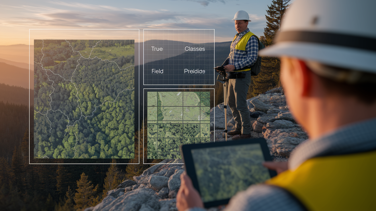
Validation compares satellite-derived forest-loss maps against independent reference data collected from field surveys, high-resolution drone imagery, or manual interpretation of finer-resolution satellite scenes. Analysts select a random or stratified sample of locations, visit them or examine them in detail, record whether the satellite classification matches reality. A confusion matrix tallies how many true forest-loss pixels were correctly detected (true positives), how many non-loss pixels were wrongly flagged (false positives, or commission errors), how many real losses were missed (false negatives, or omission errors), and how many stable pixels were correctly ignored (true negatives).
Producer accuracy measures the fraction of reference forest-loss samples that the map correctly identified, essentially the recall or sensitivity of the detection system. User accuracy measures the fraction of map-labeled loss pixels that actually were losses, the precision or reliability of a flagged alert. Overall accuracy is the percentage of all samples classified correctly, and the kappa statistic adjusts for chance agreement, providing a single metric of map quality. High kappa (above 0.8) and balanced producer/user accuracies indicate a robust detection system. Low producer accuracy means many real clearings are missed. Low user accuracy means many alerts are false alarms. Iterative refinement of thresholds, training samples, or sensor fusion strategies improves these metrics before deploying a monitoring system operationally.
| Metric | Purpose |
|---|---|
| Producer accuracy (recall) | Fraction of true forest losses correctly detected by the map; measures sensitivity to real change |
| User accuracy (precision) | Fraction of map-flagged losses that are genuine; measures reliability and false-alarm rate |
| Overall accuracy | Percentage of all validation samples classified correctly; summary measure of map performance |
| Kappa statistic | Agreement corrected for chance; accounts for class imbalance and provides single quality score |
Operational Monitoring Systems and Near‑Real‑Time Deforestation Alerts

Near-real-time monitoring systems ingest satellite imagery as soon as it’s downlinked, run change-detection algorithms within hours or days, publish alerts to web dashboards or mobile apps used by enforcement agencies, conservation groups, commodity buyers. Brazil’s DETER system processes optical and radar data from multiple satellites to flag new clearings in the Amazon every few days, triggering field inspections and legal actions against illegal loggers. Global Forest Watch aggregates data from Landsat, Sentinel, other sources into annual and weekly change layers accessible to anyone with an internet connection, democratizing access to deforestation intelligence that once required specialized expertise and infrastructure.
Google Earth Engine provides the cloud-processing backbone for many of these systems. It hosts petabytes of preprocessed satellite archives and parallelizes computations across thousands of servers. An analyst can run a change-detection algorithm over an entire country in minutes rather than weeks. Sentinel-2 and Landsat scenes are ingested automatically, preprocessed for atmospheric effects and clouds, made available in analysis-ready stacks. Hansen and colleagues used this platform to produce annual global forest-change maps at 30-meter resolution, detecting losses and gains from 2000 onward and updating the dataset each year. The workflow is now replicated by governments, NGOs, commercial monitoring services tailored to specific geographies or supply chains.
Alert workflow in a typical near-real-time system follows four stages:
Data ingestion – new satellite scenes downloaded from ground stations or cloud archives as soon as available, often within hours of acquisition.
Preprocessing – automated pipelines apply orthorectification, atmospheric correction, cloud masking, radiometric calibration to produce analysis-ready surface reflectance or backscatter.
Change detection – algorithms compare the new image against baseline mosaics or time-series models, compute change probabilities or index differences, threshold results to generate candidate alerts.
Alert publication – flagged pixels are filtered by minimum area, forest definition, user-defined regions of interest, then packaged as georeferenced polygons and pushed to web maps, email notifications, or mobile apps for field teams.
Case Examples of How Satellite Imagery Reveals Deforestation Patterns
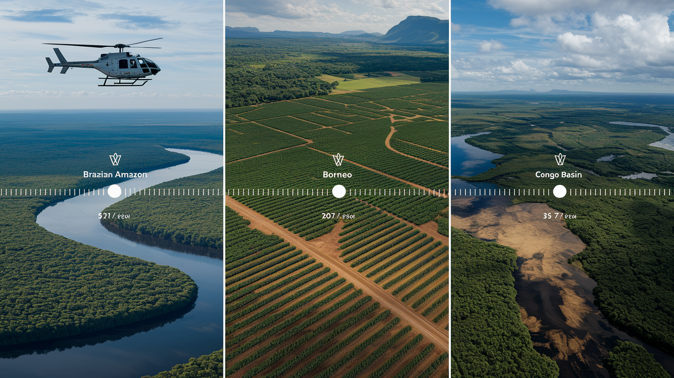
In the Brazilian Amazon, the DETER early-warning system combines optical data from Landsat and CBERS satellites with Sentinel-1 radar to detect clearings larger than a few hectares within days of occurrence. When a new patch appears, enforcement officers receive coordinates and can plan helicopter overflights or ground patrols to intercept illegal logging before the cleared timber is removed. This rapid feedback loop has been credited with reducing deforestation rates during periods of strong enforcement, though political will and funding gaps remain persistent challenges. The system’s success shows that satellite detection alone isn’t enough. Alerts must connect to responsive institutions on the ground.
Borneo and Sumatra show how time-series analysis reveals the progression of industrial plantation expansion. Analysts stack years of Sentinel-2 and Landsat imagery to trace the appearance of new roads penetrating intact forest, followed weeks or months later by systematic clearing in geometric blocks characteristic of oil-palm or pulpwood estates. Edge detection algorithms identify the straight boundaries and grid patterns that distinguish planned conversion from scattered subsistence clearing. By correlating these spatial signatures with concession maps and ownership records, supply-chain auditors can identify which companies are expanding into primary forest and apply pressure or halt sourcing to enforce zero-deforestation commitments.
In the Congo Basin, cloud cover is so persistent that optical satellites often provide only a few clear views per year. Sentinel-1 SAR fills the gap, mapping protected areas every week regardless of weather. When backscatter drops suddenly inside a national park boundary, rangers receive an alert pointing to the coordinates of suspected illegal logging. Post-detection field checks confirm that selective cutting (removing only high-value hardwoods) leaves the canopy partly intact but changes the radar return enough to trigger detection. California’s wildfire monitoring combines pre-fire Landsat baselines with post-fire MODIS thermal hotspots and Sentinel-2 burn-severity indices to map the extent of forest destroyed, guide rehabilitation priorities, track vegetation recovery over subsequent years using NDVI time series.
Limitations, Challenges, and False‑Positive Reduction in Deforestation Mapping
Cloud cover remains the primary limitation for optical sensors, especially in equatorial regions where afternoon convection generates daily thunderstorms. A Landsat or Sentinel-2 pass might capture only a sliver of usable data, forcing analysts to wait weeks for the next clear view or rely on composites that blur the timing of change. SAR mitigates this but introduces its own complexity. Backscatter is sensitive to soil moisture, surface roughness, look angle. Seasonal floods or heavy rain can mimic forest loss if baselines aren’t carefully chosen. Multi-sensor fusion, combining optical indices with SAR coherence and backscatter, improves reliability by requiring agreement across independent measurements before confirming a detection.
Seasonal phenology can resemble deforestation when deciduous trees lose leaves, grasslands brown during dry seasons, or crops are harvested. Algorithms reduce these false positives by learning annual cycles from multi-year baselines and flagging only deviations that exceed normal variability. Distinguishing plantation harvest from natural-forest clearing requires additional context: plantation boundaries, species composition, management records help classify a detected change as rotation forestry versus primary-forest conversion. High-resolution imagery reveals narrow logging roads and selective-cut gaps invisible at 30-meter resolution, but the cost and revisit limitations of commercial tasking mean this detail is reserved for priority hotspots rather than wall-to-wall monitoring. Ground truthing remains essential to calibrate thresholds, interpret ambiguous signals, confirm that automated alerts correspond to real deforestation rather than data artifacts or land-use transitions outside the scope of concern.
Future Trends in Satellite‑Based Deforestation Monitoring
Commercial satellite constellations are growing rapidly. Companies launching dozens of small optical and SAR satellites into coordinated formations. Planet’s fleet already delivers daily 3-meter imagery over the tropics, and new SAR constellations promise sub-weekly revisits at meter-scale resolution. This density of coverage will shrink detection latency from weeks to days or hours, enabling intervention before clearing progresses far. Spaceborne LiDAR systems like NASA’s GEDI provide sampled canopy-height measurements that improve biomass estimates and detect subtle degradation invisible to passive sensors. As LiDAR coverage expands and costs fall, wall-to-wall 3D forest mapping will become feasible for large regions.
Automated real-time AI systems are shifting from research prototypes to operational deployment. Cloud platforms process billions of pixels in parallel using Kubernetes-based engines that spin up thousands of virtual machines on demand, running deep-learning models that fuse optical, radar, auxiliary data into unified change probabilities. What once took a month to process for a single island now completes in hours for an entire archipelago. Integration with law enforcement, supply-chain auditing, carbon-market verification is tightening. Alerts trigger not just emails but automatic contract suspensions, field investigations, public transparency dashboards that hold actors accountable in near real time.
Key advancements shaping the next generation of monitoring:
Higher temporal and spatial resolution constellations delivering near-daily revisits at meter-scale, closing detection gaps and catching small or gradual changes.
Advanced radar and LiDAR sampling providing all-weather, day-night structure measurements that complement optical indices and improve biomass tracking.
Automated AI and cloud-native processing pipelines enabling real-time analysis of petabyte-scale archives, reducing human workload and accelerating alert delivery from detection to action.
Final Words
We jumped into the methods: satellites record visible, NIR, SWIR and radar, and canopy loss shows up as sudden drops in greenness and shifts in radar backscatter.
We covered optical indices (NDVI/EVI), SAR confirmation, time‑series records from Landsat, Sentinel‑2 and MODIS, preprocessing and change‑detection tools, plus operational alerts and case studies. Limits remain—clouds, seasonal cycles and resolution can still cause false positives.
Knowing how satellite imagery detects deforestation helps people act sooner. As sensors and AI improve, monitoring will get faster and more reliable.
FAQ
Q: How do satellites detect deforestation?
A: Satellites detect deforestation by recording multiple wavelengths; canopy loss alters spectral signatures (less green/NIR, more bare‑soil/SWIR), and abrupt, persistent drops in vegetation indices signal clearing.
Q: What role do optical sensors and NDVI/EVI play in detecting forest loss?
A: Optical sensors and indices like NDVI (near‑infrared to red vegetation index) and EVI quantify greenness; sudden index drops versus seasonal baselines indicate canopy loss while thresholds and burn checks cut false alarms.
Q: How does synthetic aperture radar (SAR) detect forest clearing and why is it important?
A: SAR detects forest clearing by measuring radar backscatter and coherence; standing forest gives high, variable backscatter, while removal lowers backscatter—so SAR provides cloud‑free, day/night confirmation of loss.
Q: Which satellite programs are commonly used to monitor forest change and what are the trade‑offs?
A: Major programs—Landsat (~30 m, 16‑day), Sentinel‑2 (10–20 m, ~5‑day), MODIS (250–500 m, daily) and commercial constellations—trade spatial resolution, revisit frequency, archive length and cost for different monitoring needs.
Q: What change detection algorithms are used to identify deforestation?
A: Change detection uses image differencing, NDVI thresholding, time‑series break methods (BFAST), continuous monitoring (CCDC) and machine‑learning classifiers (Random Forest, CNNs); time‑series approaches reduce false positives.
Q: What preprocessing and data‑cleaning steps are required before detecting forest loss?
A: Preprocessing requires orthorectification, atmospheric and radiometric correction, cloud and shadow masking, plus multi‑date compositing to normalize sensors and reduce false detections from haze or sensor differences.
Q: How is satellite‑detected forest loss validated and ground‑truthed?
A: Validation compares satellite outputs with field plots, drone surveys or very‑high‑resolution imagery; confusion matrices, producer/user accuracy, omission/commission rates and kappa statistics quantify map reliability.
Q: How do near‑real‑time deforestation alert systems work?
A: Near‑real‑time systems ingest frequent Sentinel, Landsat and SAR data, preprocess it, run automated change detection, then publish alerts that are validated for rapid response and targeted field checks.
Q: What are common limitations and causes of false positives in deforestation mapping?
A: Mapping limits include cloud cover, seasonal phenology, selective logging, burn scars and sensor resolution; using multi‑sensor fusion, seasonal baselines and time‑series checks helps reduce misclassification.
Q: What future trends will improve satellite‑based deforestation monitoring?
A: Future trends include denser commercial constellations, better SAR and LiDAR sampling, real‑time AI pipelines and cloud computing—improving detection speed, canopy‑height change measurement and small‑scale disturbance tracking.
Q: What physical signals in satellite data reveal deforestation?
A: Physical signals revealing deforestation include NDVI drops, SWIR increases, rising bare‑soil reflectance, reduced SAR backscatter, and thermal anomalies from fires.