
How can we know what a star or planet is made of when we can’t touch it?
Astronomers do it by splitting its light into a spectrum and reading absorption and emission lines—chemical fingerprints.
They use spectrographs, lab catalogs, and careful calibration to lock line positions down to real wavelengths.
Then they match sets of lines and model temperature and ionization (atoms losing electrons) so strength differences tell what and how much is present.
This post walks through those steps, explains why single lines can mislead, and points out the key checks that keep identifications reliable.
Core Principles Behind Identifying Composition from Spectra

A spectrograph splits incoming starlight by sending it through a prism or diffraction grating, spreading the light across a detector the same way a raindrop turns sunlight into a rainbow. What you get is a spectrum dotted with narrow dark gaps called absorption lines, where atoms and molecules in the star’s outer layers grabbed photons at very specific wavelengths. Hot, low-density gas clouds flip the script: they make bright emission lines at those same wavelengths where cooler foreground gas would absorb. Both kinds of lines work like chemical barcodes. Each element and molecule stamps its own unmistakable pattern.
Every chemical element owns a unique set of wavelengths because its electrons sit in discrete energy levels, shaped by how many protons are in the nucleus and the quantum rules that govern electron orbits. When an electron absorbs a photon with exactly the right energy, it jumps to a higher level. When it drops back down, it kicks out a photon at that same wavelength. Hydrogen’s Balmer series gives you absorption lines at Hα (656.28 nm), Hβ (486.13 nm), and shorter wavelengths. Helium, calcium, iron, every other element, they all add their own fixed patterns. Because these wavelengths never budge for a given element, astronomers can figure out what a star or planet is made of by measuring where the lines land and checking those positions against lab catalogs.
Matching one line can be sketchy. Two different elements might park lines close together. So astronomers always hunt for the full fingerprint. They cross-check several lines from the same element, confirm the pattern spacing matches lab data, and use how strong the lines are from different ionization states to lock in the ID. This pattern-matching trick turns a spectrum from a simple intensity plot into a detailed grocery list of which atoms and molecules are hanging out in the distant object.
Absorption lines show up as dark notches when a continuous background shines through cooler gas. Emission lines glow bright when hot, spread-out gas radiates straight at you. Each element’s electron setup makes a fixed set of transition wavelengths that never changes. Measured wavelengths from astronomical spectra get matched against precise lab measurements to pin down which element you’re looking at. Lining up several lines from the same element clears up any confusion and confirms it’s really there. The spacing, number, and layout of lines in a series tell you which element made them, no matter what any single line says.
Spectroscopic Formation of Absorption and Emission Signatures
At the atomic level, spectra happen because electrons only occupy certain allowed energy levels, labeled by quantum numbers like n = 1, 2, 3, and so on. An electron chilling in a lower energy state can grab a photon whose energy exactly matches the gap to a higher level, which kicks the electron into that excited state. A moment later the electron falls back, tossing out a photon of the same energy and wavelength in a random direction. When we look at a star, the smooth spectrum from deep hot layers passes through cooler outer gas. Atoms in that gas snatch photons heading our way at their go-to wavelengths, carving out dark absorption lines. If instead we’re watching a hot nebula against empty space, we only see the photons dumped out as electrons tumble down through energy levels. Bright emission lines on a dark backdrop.
Hydrogen lays it out clearly. The Balmer series matches transitions where electrons drop to or get excited from the n = 2 level. The Lyman series taps the ground state (n = 1) and churns out ultraviolet lines. The Paschen series kicks off at n = 3 and delivers infrared features. Each series follows a math pattern set by the energy-level structure. Once you spot Hγ at 434.05 nm and Hδ at 410.17 nm alongside Hα and Hβ, you’ve nailed hydrogen and sketched out part of its quantum ladder. Other elements with messier electron shells make more tangled patterns, but the physics stays the same. Quantized energy jumps turn straight into discrete spectral lines.
Spectral Patterns and Element Identification Techniques

Identifying an element means spotting the full set of lines it makes, not leaning on a single wavelength. A spectrum jammed with hundreds of narrow features calls for pattern-matching software and reference books to sort out overlapping contributions. Astronomers measure the wavelengths of all the big lines, then comb through lab databases for sets that match the observed spacings and relative punch. When multiple lines from a series pop up at their expected spots—say, four Balmer lines of hydrogen or the doublet shape of neutral sodium—you’ve locked it down. One line might accidentally sit on top of a feature from another element, but the full pattern wipes out that headache.
Metal-rich stars (astronomers call anything heavier than helium a “metal”) throw up dense thickets of absorption lines because elements like iron, nickel, and titanium each dump dozens or hundreds of transitions across the visible and near-infrared. These packed spectra need high spectral resolution to pull individual lines apart, and careful modeling to tag each feature to the right element. In very cool stars, molecules like titanium oxide (TiO) form in the photosphere and slice out broad absorption bands—clusters of tightly packed lines that smear into wide, shallow dips. These molecular bands work as temperature gauges and show that complicated chemistry is running in the star’s outer layers.
| Element/Ion | Key Wavelength Feature |
|---|---|
| Hydrogen (H I Balmer) | Hα at 656.28 nm, Hβ at 486.13 nm |
| Helium I (neutral) | He I line at 587.56 nm |
| Calcium II (singly ionized) | Ca II H & K doublet at 393.37 nm and 396.85 nm |
Spectrograph Instrumentation and Data Calibration
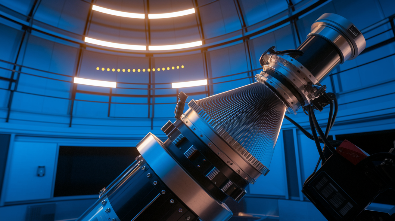
A modern astronomical spectrograph sticks a narrow slit at the telescope’s focal plane, letting light from a single star or a thin slice of a nebula slip in. That light then hits a dispersing element (either a prism or a diffraction grating) which bends different wavelengths by different amounts, fanning the spectrum across a detector. High-resolution gear uses echelle gratings and cross-dispersers to cram many spectral orders onto a two-dimensional chip, hitting resolving powers R (λ divided by the smallest resolvable wavelength gap Δλ) from 10,000 up to 100,000 or higher. Lower-resolution survey spectrographs swap detail for speed, grabbing broad features and molecular bands at R around a few hundred to a few thousand.
Before any real measurements happen, the raw detector counts need to turn into calibrated wavelength and flux. Observers light up the spectrograph with a calibration lamp (often thorium-argon, ThAr) which spits out a dense comb of emission lines at exactly known wavelengths. Software fits a polynomial or spline that maps pixel spots to wavelengths, building the wavelength solution. Flat-field exposures fix pixel-to-pixel sensitivity wobbles, and bias frames strip out electronic offsets. Only after these steps can astronomers trust that a measured line position matches a real physical wavelength instead of some instrument quirk.
Flat-fielding means you divide the science spectrum by a uniform-illumination shot to knock out pixel sensitivity shifts and fix vignetting. Bias subtraction pulls the electronic baseline signal the detector’s readout adds before any light shows up. The wavelength solution fits calibration-lamp line spots to known wavelengths, giving you a function that converts pixel coordinates to nanometers or angstroms. Using calibration lamps like ThAr, neon, or other emission sources gives stable reference lines across the full wavelength stretch. Checking resolving power means measuring the full-width at half-maximum of calibration lines to confirm the instrument hands you the expected R and catch focus or alignment trouble. Verifying spectral linearity confirms that wavelength steps per pixel hold steady or track the expected grating equation across the detector.
Temperature, Ionization, and Their Effects on Spectral Composition Analysis
How strong a spectral line looks depends not just on how much of an element is there, but on how many atoms are parked in the right energy level to absorb or spit out light at that wavelength. The Boltzmann distribution runs the population of excited states: hotter gas shoves more atoms into higher energy levels, beefing up lines that start from those states and weakening ground-state transitions. At the same time, higher temps ionize more atoms, ripping away electrons and changing which spectral series show up. The Saha equation puts numbers to this ionization balance, predicting what fraction of an element exists as neutral atoms, singly ionized ions, doubly ionized ions, and so on, for a given temperature and pressure.
Cecilia Payne’s 1925 doctoral work proved that hydrogen and helium run the show in stellar composition by mass, even though their lines don’t always hog the spectrum. In cooler stars, hydrogen’s Balmer lines are wimpy because most hydrogen atoms stay in the ground state (n = 1), and Balmer absorption needs electrons starting in n = 2. Hotter A-type stars flash the strongest Balmer lines because their temps fill the n = 2 level nicely. Even hotter O and B stars ionize most of their hydrogen, so neutral-hydrogen lines fade and helium lines (including singly ionized helium in the hottest cases) step in. This temperature-driven shuffle means you can’t just assume a strong line signals high abundance. You’ve got to model the physical conditions to pull apart temperature and ionization effects from the actual chemical recipe.
Modern abundance work fits model stellar atmospheres to observed spectra, tweaking temperature, surface gravity, and element abundances until the fake spectrum matches the data. Local thermodynamic equilibrium (LTE) assumes collisions beat out radiation in setting energy-level populations, which makes the math simpler. When radiation matters (common in hot stars or stretched-out atmospheres), non-LTE modeling handles how photons drain certain levels and mess with line strengths. Skipping these effects can throw abundance guesses off by factors of two or more.
Measuring Chemical Abundances from Spectra

Once you’ve tagged which lines belong to which elements and fixed for temperature and ionization, you measure the line strength to figure out how much of each element is sitting there. The equivalent width (the width of a perfectly dark rectangle with the same total area as the observed absorption line) sizes up line strength in a way that doesn’t care about the continuum level. Weak lines grow in a straight shot with abundance, but strong lines max out, meaning their centers go totally dark and piling on more atoms only spreads the wings. To wrangle this nonlinear mess, astronomers use curves of growth or full spectral synthesis, which cooks up a fake spectrum from a model atmosphere, atomic line data (including oscillator strengths and damping constants), and a guess at abundances, then fiddles those abundances until the model lines up with what’s observed.
Spectral synthesis handles line blending, continuum shape, and the nitty-gritty physics of how lines form, making it the top pick for abundance work. The whole thing needs solid atomic data: each transition’s oscillator strength (tied to its built-in odds) and wavelength must come from lab measurements or quantum math. Slop in these values rolls straight into the final abundances, so double-checking multiple lines of the same element and comparing results from different ionization stages gives you crucial error bars and sanity checks.
Equivalent width measurement means you add up the absorption profile to get a single number (in milliangstroms or angstroms) for line strength, which then plugs into curve-of-growth or model-atmosphere work. Using oscillator strengths (atomic transition odds, or log gf values) converts measured line strengths into column densities or abundances. Errors in gf flow straight through to abundance errors. Synthetic spectral fitting computes a full model spectrum over a wavelength slice, varies parameters (temperature, abundances, microturbulence), and shrinks the gap between model and what you see. Error propagation pulls together uncertainties from continuum placement, wavelength calibration, atomic data, model-atmosphere settings, and line blending to hand you realistic confidence spreads on abundances.
Motion and Broadening Effects in Spectral Interpretation
Every spectral line shows up Doppler-shifted if the source is cruising toward or away from us. The wavelength shift follows Δλ/λ = v/c, where v is the speed along our line of sight and c is the speed of light (299,792,458 m/s). A star heading away gives you a redshift (lines slide to longer wavelengths). Stuff coming closer blueshifts its lines. Before stacking observed wavelengths against lab rest values, astronomers clock this shift (often from many lines at once) and drag all wavelengths back to the rest frame. The same Doppler math lets us clock rotation: one edge of a spinning star moves toward us and the other away, stretching every line into a profile whose width spills the projected rotation speed.
Beyond bulk motion, several physical things widen spectral lines on their own. Thermal broadening pops up because atoms jiggle randomly at speeds set by temperature. Hotter gas or lighter atoms make wider lines. Pressure (collisional) broadening kicks in when smacks from neighboring atoms mess with energy levels during a transition, and it gets worse in denser atmospheres. Turbulent flows (convective bubbles or shock waves) toss in extra Doppler broadening. Magnetic fields split lines into multiple pieces through the Zeeman effect, and strong fields can totally reshape line profiles. Measuring and modeling these broadening tricks reveals temperature, density, magnetic-field strength, and motion, turning line shapes into a deep diagnostic beyond simple yes-or-no chemistry.
Practical Examples of Identifying Stellar and Planetary Composition
When you crack open a stellar spectrum, the first things that catch your eye are usually the hydrogen Balmer lines. Hα at 656.28 nm and Hβ at 486.13 nm are bright and hard to miss in early-type stars. Helium’s neutral line at 587.56 nm (He I) shows up in hotter stars, while the singly ionized helium line He II at 468.6 nm screams extremely high temps you find in O-type stars. Cooler stars and planets wave around strong molecular absorption: carbon monoxide (CO) and titanium oxide (TiO) bands take over M-dwarf spectra, and water vapor, methane, and carbon dioxide features blow the whistle on the atmospheric chemistry of exoplanets and brown dwarfs. Nebulae toss in forbidden lines (transitions that only fire in super low-density gas) like doubly ionized oxygen [O III] at 500.7 nm, which never pop up in lab conditions but blaze in interstellar space.
Hydrogen Balmer series (Hα, Hβ, Hγ, Hδ) rules in A-type stars. Hα at 656.28 nm is the brightest and the go-to diagnostic for stellar rotation, winds, and stuff falling in. Helium He I at 587.56 nm tags moderately hot stars (B and early A). How strong it looks next to hydrogen lines pins down effective temperature. Calcium II H & K doublet throws strong resonance lines at 393.37 nm and 396.85 nm. They’re touchy about chromospheric action and stellar age in cool stars. Sodium D doublet parks a pair of lines near 589.0 nm and 589.6 nm. They’re everywhere in stellar photospheres and exoplanet transmission spectra. Iron lines scatter hundreds of Fe I and Fe II features across the optical. They’re the backbone for metallicity work and stellar-population studies. Titanium oxide (TiO) bands carve broad molecular dips in M-type stars. How deep they go climbs with cooler temp and gets used to sort spectral subclasses. Carbon monoxide (CO) overtone bands sit in near-infrared in cool giants and brown dwarfs. CO strength traces the carbon-to-oxygen ratio and temperature. Forbidden [O III] and [N II] lines glow in planetary nebulae and H II regions. Their intensity ratios decode electron temperature, density, and ionization state in spread-out gas.
Final Words
Right in the action: telescopes feed starlight into spectrographs that spread it into absorption and emission lines, and those patterns get matched to lab wavelength lists to name elements and molecules.
Accurate IDs need careful calibration, motion and broadening corrections, and models that include temperature and ionization; abundance comes from line strengths or full spectral fitting.
If you still wonder “how do astronomers determine composition from spectra”, the short answer is: match fingerprints, confirm with multiple lines, and fit conditions. It’s a reliable way to read chemical stories in light—and we’ll keep learning more.
FAQ
Q: How can astronomers use spectra to determine the composition of stars and the Sun, and how do different spectra help?
A: Astronomers use spectra to determine the composition of stars and the Sun by dispersing starlight into absorption or emission lines, matching unique wavelength fingerprints to laboratory lists, and measuring line strengths while correcting for temperature and ionization.
Q: How do scientists know the composition of planets?
A: Scientists know the composition of planets by analyzing reflected, transmitted, and thermal spectra to identify molecular bands, using transit spectroscopy for atmospheres, and combining lab matches with mass–radius data or in situ probe measurements.