
Can a satellite really measure ocean height to millimeters from 1,330 kilometers up?
Yes, by firing microwave pulses straight down and timing the echo.
Radar altimeters turn that travel time into a range, then subtract the satellite’s orbit to get sea surface height.
After correcting for atmosphere, waves, and tides, repeated measurements from missions like TOPEX/Poseidon, the Jason series, and Sentinel-6 reveal a steady rise of about 3.3 millimeters per year.
This post shows how the radar trick works, why it’s so precise, and which satellites keep the climate record continuous.
Core Satellite Methods Used for Tracking Sea Level Change
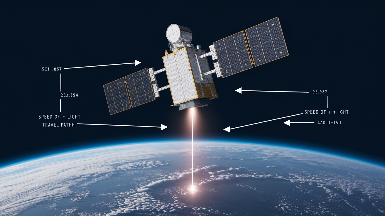
Satellites track sea level by pointing radar altimeters straight down at the ocean and timing how long a microwave pulse takes to bounce back. That round-trip tells you the distance between the satellite and the water surface. Radio waves move at the speed of light, so the math is simple: divide travel time by two, multiply by light speed, and you’ve got range. Subtract that from the satellite’s orbit height and you get sea surface height above Earth’s center.
Modern radar altimetry hits about 2 to 3 centimeters of vertical precision on a single shot after corrections. Doesn’t sound like much. But average thousands of measurements over months and years, and patterns show up with millimeter confidence. The real strength comes from repeating the measurement over the same ocean patch every ten days or so, building a time series that shows whether water is rising, dropping, or holding steady.
TOPEX/Poseidon kicked off the continuous satellite record in 1992. Jason-1 took over in 2001, Jason-2 in 2008, Jason-3 in 2016, and Sentinel-6 Michael Freilich in 2020. Each handoff was managed carefully so the new satellite could fly alongside the old one, cross-checking before the older mission shut down. This unbroken chain since 1992 lets scientists say with confidence that global mean sea level climbs about 3.3 millimeters per year, and it’s accelerating.
The basic workflow:
- Emit a radar pulse – Altimeter sends a short microwave burst toward the ocean.
- Measure echo return time – Instrument records how long the reflection takes to come back.
- Apply corrections – Atmospheric delays, wave height, other factors get removed mathematically.
- Compute sea surface height – Subtract corrected range from the satellite’s orbit position to find absolute height above the reference ellipsoid.
Radar Altimetry Techniques Behind Satellite Sea Level Monitoring

When the radar pulse hits water, it doesn’t bounce back clean. The return signal spreads out in time because the ocean is rough, covered in slopes and foam. The altimeter samples this return waveform, a curve that peaks as more of the pulse reflects, then fades as the signal moves past the brightest part of the wave. By analyzing the waveform’s shape, scientists pull out the exact moment the leading edge crossed the mean sea surface, giving sharper range than a simple time stamp would.
That waveform also carries wave height and wind speed information. Calm water produces a sharp return. Choppy seas stretch the signal. This extra detail helps correct for sea-state bias, a subtle error that happens because wave troughs and crests don’t reflect radar equally. Getting range right to the centimeter depends on understanding these waveform features:
- Leading edge rise time – How fast the signal climbs tells you wave slope and roughness.
- Peak amplitude – Stronger peaks suggest calmer conditions or better geometry.
- Trailing edge decay – Tail shape indicates off-nadir reflections and wave structure.
- Noise floor – Background scatter sets the lower limit of detectable change.
- Retracking point – Algorithms pick the exact spot on the leading edge representing the mean surface.
Atmospheric and Sea-State Corrections
Even after you pull a clean range from the waveform, you’re not done. The microwave pulse slows down passing through charged particles in the ionosphere and water vapor in the troposphere. Ionospheric delay can add several centimeters of error depending on solar activity and time of day. Most modern altimeters transmit at two frequencies, Ku-band and C-band, so the difference in delay reveals how much the ionosphere bent the signal. A correction model removes that bias.
Water vapor in the lower atmosphere, especially over warm tropical oceans, causes wet tropospheric delay. Satellites carry microwave radiometers that measure column water content, then apply a physics-based correction for slower propagation. Dry air also slows the signal slightly, but that delay is predictable and gets removed with a standard atmospheric pressure model.
Sea-state bias is trickier. Wind-driven waves scatter radar differently depending on whether you’re measuring a trough or a crest, and the altimeter tends to see troughs more clearly. Result is a small negative bias, typically a few centimeters, varying with wave height and wind speed. Empirical models, tuned with buoy data and past missions, adjust each measurement based on waveform shape.
Tides add another layer. Ocean tides can move the surface up or down by meters, and even solid-Earth tides shift the ocean floor. Both have to be predicted with tide models and subtracted so measured height reflects long-term change, not the rhythmic pull of Moon and Sun.
Key Satellite Missions Providing Sea Level Records
The continuous satellite sea level record starts with TOPEX/Poseidon, a joint NASA and French space agency mission launched August 10, 1992. TOPEX/Poseidon proved radar altimetry could deliver global ocean height measurements stable enough to catch slow climate trends. The mission ran until 2006, overlapping with its successor to avoid gaps or drift.
Jason-1 launched December 7, 2001, carrying an improved altimeter and flying the same orbital track as TOPEX/Poseidon during calibration. That overlap let scientists compare the two instruments directly, adjusting for any bias before TOPEX/Poseidon retired. Jason-2, also called OSTM (Ocean Surface Topography Mission), followed June 20, 2008, adding better tracking systems and continuing the ten-day repeat cycle. Jason-3 launched January 17, 2016, still operating as of 2020, maintaining the reference orbit while newer platforms come online.
Sentinel-6 Michael Freilich launched November 21, 2020, carrying the Poseidon-4 altimeter, which uses synthetic aperture radar processing to sharpen along-track resolution and cut noise. A second Sentinel-6 satellite, Sentinel-6B, is scheduled for 2025 to push the record past 2030. When Sentinel-6 and Jason-3 flew side by side, their measurements agreed to within 2 millimeters, confirming the new instrument could be stitched seamlessly into the climate data record.
| Mission | Launch Year | Contribution |
|---|---|---|
| TOPEX/Poseidon | 1992 | Established the modern altimetry era and first continuous global record. |
| Jason-1 | 2001 | Extended the time series with improved tracking; overlapped TOPEX for calibration. |
| Jason-2 (OSTM) | 2008 | Enhanced orbit determination and continued the reference track. |
| Jason-3 | 2016 | Maintained the ten-day cycle; still operating alongside Sentinel-6. |
| Sentinel-6 MF | 2020 | SAR altimetry for higher resolution; cross-calibrated with Jason-3 to <2 mm. |
How Satellite Orbits Enable Accurate Sea Level Measurements

Knowing ocean height means nothing unless you know exactly where the satellite is. Jason-class missions fly at about 1,330 kilometers above Earth’s surface, and their position must be nailed down to a few centimeters in all three dimensions. That precision comes from three tracking systems working together: GPS receivers onboard the satellite, ground-based laser ranging stations, and DORIS (Doppler Orbitography and Radiopositioning Integrated by Satellite).
GPS gives continuous position updates by comparing signals from the navigation constellation. Satellite laser ranging stations on the ground fire short laser pulses at retroreflectors on the satellite, measuring round-trip time to pin down range with millimeter accuracy. DORIS uses a network of ground beacons emitting radio signals. The satellite measures Doppler shifts as it passes overhead, constraining velocity and orbit shape. Fusing all three data streams, orbit analysts produce a precise orbit determination solution, good to about 1 to 2 centimeters radially.
The orbit itself is designed to repeat the same ground track every 9.9156 days, nearly exactly ten days. This repeat cycle means the satellite samples the same strips of ocean over and over, letting scientists build time series at each crossing point. Between crossings, Earth rotates underneath, so ground tracks spread out and eventually cover the global ocean between about 66 degrees north and south latitude.
Three orbit-determination systems enable centimeter positioning:
- GPS receivers – Provide real-time three-dimensional position by tracking multiple navigation satellites.
- Satellite laser ranging – Ground stations pulse lasers at onboard reflectors for millimeter-precision range checks.
- DORIS beacons – Measure Doppler shifts of radio signals to refine velocity and height estimates.
Processing Satellite Data Into Reliable Sea Level Trends

Raw altimeter data is just a stream of ranges and waveforms. Turning that into a sea level trend takes a pipeline of corrections, transformations, and quality checks. First, ionospheric and tropospheric corrections adjust the measured range for atmospheric effects. Then tidal models subtract predicted height change from ocean tides, solid-Earth tides, and pole tides. Sea-state bias and inverse barometer corrections account for wave roughness and atmospheric pressure loading. What’s left is a corrected range that, when subtracted from precise orbit height, gives you sea surface height relative to a reference ellipsoid, a smooth mathematical model of Earth’s shape.
Sea surface height on its own isn’t very useful for climate work because Earth’s gravity field is lumpy. The geoid, the surface where gravity potential is constant, undulates by tens of meters. Ocean currents and density variations add dynamic topography on top. To isolate the climate signal, scientists subtract a long-term mean sea surface, leaving sea level anomaly, the deviation from average. SLA gets gridded, averaged, and tracked over time.
Along-track measurements are dense, spaced every few kilometers, but they’re just lines on the ocean. To make maps, processing centers bin data into grid cells, typically 0.25 degrees or coarser, and apply space-time interpolation to fill gaps between tracks. Monthly averages smooth out short-lived features like weather and eddies. Global mean sea level comes from averaging all grid cells, weighted by area, and stacking those monthly values into a time series. Trends get estimated by fitting a line or more complex model to the time series, accounting for seasonal cycles and occasional jumps from volcanic eruptions or El Niño events.
From Raw Range to Sea Level Anomaly
Each step in the transformation has to happen in the right order or errors compound. Standard sequence:
- Record raw altimeter range and waveform – Instrument saves two-way travel time and waveform shape for each pulse.
- Retrack the waveform – Algorithms find the precise point on the leading edge corresponding to mean sea surface.
- Apply geophysical and atmospheric corrections – Ionosphere, troposphere, tides, sea-state bias, and pressure loading get removed from range.
- Compute corrected sea surface height – Subtract fully corrected range from satellite orbit height above reference ellipsoid.
- Remove mean sea surface to form anomaly – Subtract multi-year average height at that location, leaving sea level anomaly that tracks change over time.
Data quality flags mark measurements affected by rain, ice, or land contamination, and those points get excluded from climate products. What remains is a gridded, validated dataset ready for trend analysis, uploaded to archives where researchers and forecasters pull it for everything from ocean modeling to coastal planning.
Monitoring Climate Drivers Behind Sea Level Rise Using Satellites

Sea level doesn’t rise uniformly because the ocean isn’t a bathtub. Two main processes push the surface higher: thermal expansion, where warming water takes up more volume, and mass addition from melting ice on land. Satellite altimetry measures total height change, but separating the two contributions requires extra information. That’s where gravity missions like GRACE (Gravity Recovery and Climate Experiment) come in. GRACE tracks tiny changes in Earth’s gravitational field caused by shifting mass, whether that’s ice melting off Greenland or water moving from land to ocean.
When GRACE detects mass loss over an ice sheet, you know meltwater is flowing into the ocean, raising sea level by adding volume. Altimetry sees the combined effect, thermal plus mass, so subtracting the GRACE-derived mass signal leaves the steric (density-driven) component, mostly thermal expansion. This attribution matters because ice melt is less reversible than thermal changes. If polar ice sheets keep shedding mass, sea level rise accelerates in ways that warming alone wouldn’t cause.
The ocean has absorbed more than 90 percent of excess heat trapped by greenhouse gases since 1970, and that heat penetrates deep. Measurements from profiling floats and ship surveys show record ocean heat content down to 2,000 meters. As that warmth spreads, top layers expand, lifting the surface. Altimetry integrates this expansion across the global ocean, giving a direct measure of how much warming has raised sea level so far.
Four major contributors in the satellite record:
- Thermal expansion – Warming seawater expands, raising the surface without adding mass.
- Greenland ice sheet melt – Accelerating discharge and surface melt send freshwater to the North Atlantic.
- Antarctic ice sheet loss – Thinning glaciers and ice-shelf collapse contribute mass to the Southern Ocean.
- Mountain glacier retreat – Thousands of small glaciers worldwide lose volume, adding water globally.
Regional and Seasonal Variations in Satellite-Measured Sea Levels

Global mean sea level tells you the planet-wide average, but the ocean doesn’t rise evenly. Some regions climb at 10 millimeters per year or more, while others stay flat or even drop slightly over the same period. These differences come from ocean currents redistributing heat and water, wind patterns piling water against coastlines, and variations in salinity and temperature changing water density. Satellite altimetry captures this patchwork because it samples the entire ocean, not just a few coastal tide gauges.
Dynamic topography, the height difference caused by currents and pressure gradients, shifts with climate modes like El Niño and La Niña. During El Niño, warm water sloshes east across the Pacific, raising sea level near South America and dropping it in the western Pacific. Altimeters see these swings clearly, month by month, as anomalies reaching tens of centimeters locally. Over decades, persistent wind changes or current shifts leave a regional trend much larger or smaller than the global average.
Seasonal cycles show up too. Thermal expansion peaks late summer when the upper ocean warms, then contracts in winter. Rainfall and river discharge change ocean mass seasonally, especially near large deltas. Altimetry data averaged over a year smooths these cycles, but monthly maps reveal the breathing pattern of the ocean as it heats, cools, and exchanges water with atmosphere and land.
Three factors driving uneven sea level patterns:
- Ocean current variability – Changes in strength or path of currents like the Gulf Stream shift water height regionally.
- Wind stress and atmospheric pressure – Persistent wind patterns pile water up or push it away from coastlines.
- Climate oscillations – El Niño, the Pacific Decadal Oscillation, and the North Atlantic Oscillation redistribute heat and water on multi-year timescales.
Integrating Satellites With Tide Gauges and Ground-Based Systems

Tide gauges have measured sea level for more than a century, providing the longest records we have. But they’re stuck on coastlines, and coastlines aren’t evenly distributed. Europe, Japan, and parts of North America have dense networks. The central Pacific and much of the Southern Hemisphere have big gaps. That geographic bias made it hard to calculate a true global average before satellites arrived. Tide gauges also measure relative sea level, the height of water compared to land, which can move up or down on its own due to subsidence, sediment compaction, or post-glacial rebound.
Satellites measure absolute sea level relative to Earth’s center, so they don’t care if land is sinking. But that difference makes direct comparison tricky. To cross-check satellite and tide gauge data, scientists install GPS receivers at gauge sites to track vertical land motion. Subtract land movement from the tide gauge record, and you get absolute sea level that should match the satellite measurement at that location. When the two agree within a few millimeters, it confirms satellite corrections and calibrations are working.
This cross-validation also stabilizes the long-term satellite record. Tide gauges drift slowly due to instrument aging or benchmark shifts, and satellites can have subtle orbit errors or sensor degradation. By anchoring both to GPS and to each other, processing centers detect and correct drifts that would otherwise corrupt the climate trend. The combination gives you the best of both worlds: spatial coverage of satellites and the long temporal baseline of tide gauges, merged into a single consistent dataset.
Vertical Land Motion and Its Importance
Land doesn’t sit still. In places like the Gulf Coast or river deltas, ground sinks as sediment compacts or as oil and water get extracted. In Scandinavia and Canada, the crust is still rebounding after ice sheets melted at the end of the last ice age, lifting land a few millimeters per year. For a tide gauge, sinking land looks like rising sea level, and rising land looks like falling sea level. GPS measurements separate the two signals, letting you isolate the ocean’s contribution. Without that correction, you’d misinterpret local flooding risk and blend land motion into the climate record, biasing the global trend.
How Satellite Sea Level Data Supports Coastal Risk and Planning

Coastal planners need to know how high and how fast water will rise in their specific region, not just the global average. Satellite altimetry provides regional maps and trend estimates that feed into flooding risk assessments and infrastructure design standards. By combining historical satellite data with tide gauge records and climate projections, models can estimate storm surge heights under future sea levels, showing which neighborhoods will flood during a hurricane twenty or fifty years from now.
Regional sea level trends also help prioritize adaptation spending. A coastline experiencing 8 millimeters per year of rise needs levees, beach nourishment, or managed retreat sooner than one seeing 2 millimeters per year. Altimetry data, updated every month, tracks whether the local rate is steady, accelerating, or responding to climate oscillations. That real-time monitoring lets agencies adjust plans as conditions change, rather than relying on static projections that might’ve been made a decade ago.
Long-term projections depend on understanding mechanisms behind the rise. The IPCC’s latest assessment reports a global rise of 0.20 meters between 1901 and 2018, with the rate climbing to 3.7 millimeters per year for 2006–2018. Under various shared socioeconomic pathways, models project an additional 1.0 to 1.7 meters by 2150. Satellite records anchor these projections by providing the recent baseline and revealing how quickly acceleration is happening.
| Use Case | Data Source | Purpose |
|---|---|---|
| Storm surge analysis | Satellite altimetry + tide gauges | Model peak flood heights under elevated baseline sea level. |
| Regional planning | Gridded sea level anomaly maps | Identify high-risk zones and prioritize infrastructure investments. |
| Long-term projections | Multi-decadal satellite trends + climate models | Estimate future sea level rise for policy and design standards. |
Emerging Technologies Enhancing Satellite Sea Level Monitoring
Sentinel-6’s Poseidon-4 altimeter marks a step forward by using SAR, or synthetic aperture radar, processing. Traditional altimeters average returns over a footprint several kilometers across. SAR mode sharpens along-track resolution to a few hundred meters by coherently combining multiple pulses, like how a photographer uses a longer exposure to gather more light. Result is lower noise and better ability to resolve small-scale features like coastal eddies or narrow straits, areas that older missions struggled to measure cleanly.
Machine learning is starting to show up in the processing pipeline. Algorithms trained on years of waveform data can recognize subtle patterns indicating rain contamination, sea ice edges, or unusual wave conditions, flagging those measurements automatically. Other models fuse altimetry with sea surface temperature, ocean color, and atmospheric reanalysis to fill gaps between satellite tracks, producing higher-resolution maps than interpolation alone would allow. These techniques don’t replace the physics, but they help squeeze more information out of observations we already have.
Continuity remains the biggest challenge. A single satellite gives you snapshots. An unbroken series gives you a climate record. Sentinel-6B, planned for 2025, will ensure overlap and redundancy through at least 2030. Beyond that, space agencies are designing next-generation systems with wider swaths, multi-frequency altimeters, and on-board processing to deliver data faster. The goal is a future where sea level monitoring is as routine and reliable as weather satellites, with multiple platforms cross-checking each other and no risk of a gap that would break the trend line.
Four technologies shaping the next decade of sea level monitoring:
- SAR altimetry – Synthetic aperture processing improves along-track resolution and reduces measurement noise.
- Multi-satellite fusion – Combining data from several missions increases spatial and temporal coverage.
- Machine learning anomaly detection – Automated quality control flags contaminated data and improves gridded products.
- On-board real-time processing – Faster data delivery supports operational ocean forecasting and early-warning systems.
Final Words
In the action, satellites ping the ocean, time the echo, and turn those times into sea surface height measurements with centimeter precision.
We ran through radar altimetry, precise orbits, major missions, data processing, and how gravity and warming show where the extra water comes from.
Those satellite records get checked against tide gauges and feed planning tools for coastal risk.
If you want a simple takeaway: understanding how satellites monitor sea level rise helps communities prepare with clearer maps and better forecasts — and steady measurements make better choices possible.
FAQ
Q: How do satellites measure sea level?
A: Satellites measure sea level by sending microwave pulses to the ocean, timing the echo to get range, then subtracting that range from the satellite’s precisely known orbit height to get sea surface height.
Q: What corrections are needed for radar altimetry?
A: Radar altimetry needs corrections for atmospheric delays (ionosphere, water vapor), sea‑state bias, tides, and other geophysical effects so raw echo times become accurate sea surface heights.
Q: Which satellite missions provide long-term sea level records?
A: The long-term sea level record comes from TOPEX/Poseidon (1992), Jason‑1 (2001), Jason‑2 (2008), Jason‑3 (2016), and Sentinel‑6 Michael Freilich (2020), giving near-continuous coverage since 1992.
Q: How accurate are satellite sea level measurements?
A: Modern altimeters achieve about 2–3 cm vertical precision per measurement; after calibration and cross-comparison, Sentinel‑6 and Jason‑3 agree to under about 2 mm.
Q: How do orbit systems enable accurate measurements?
A: Precise orbits come from GPS, DORIS, and satellite laser ranging, which fix satellite position to centimetre precision; subtracting range from orbit height yields accurate sea surface height, with ~10‑day repeats.
Q: How are raw altimeter ranges processed into usable sea level data?
A: Raw ranges are corrected for atmosphere and tides, the geoid or mean sea surface is removed, sea level anomalies are computed, and values are averaged into monthly maps and long‑term trends.
Q: How do satellites separate sea level rise causes like thermal expansion and ice loss?
A: Satellites separate causes by combining altimetry (surface height) with gravity missions like GRACE (mass changes); thermal expansion shows as volume-driven height changes, ice loss shows as mass-driven gravity signals.
Q: How do regional and seasonal variations show up in satellite data?
A: Regional and seasonal variations appear as differing rates and patterns—dynamic topography, currents, and El Niño move water around, producing local rates roughly from 3 to 10 mm per year and seasonal swings.
Q: How are satellites and tide gauges integrated and calibrated?
A: Satellites and tide gauges are cross‑calibrated using overlapping records and coastal GPS to correct vertical land motion, aligning coastal relative sea level with satellite absolute heights for climate quality data.
Q: How does satellite sea level data help coastal planning and risk?
A: Satellite sea level data feed storm surge models, map regional flooding risk, and inform long‑term projections used in coastal planning, adaptation decisions, and policy assessments like IPCC scenarios.
Q: What new technologies are improving satellite sea level monitoring?
A: New advances include Poseidon‑4 SAR altimetry for finer resolution, multi‑satellite data fusion, machine learning for anomaly detection, and Sentinel‑6B for continuity planned around 2025.