
What if the thing stopping us finding Earth twins isn’t our telescopes but our wavelength ruler?
Laser frequency combs are that ruler: a grid of very stable light lines tied to atomic clocks that let high-resolution spectrographs measure Doppler shifts down to about 10 centimeters per second, roughly walking speed.
In this post I’ll show how combs are made, locked, coupled into spectrographs, and used in calibration sequences so you can turn raw spectra into reliable radial velocities for exoplanet detection.
How Laser Frequency Combs Enable Ultra‑Precise Radial Velocity Calibration
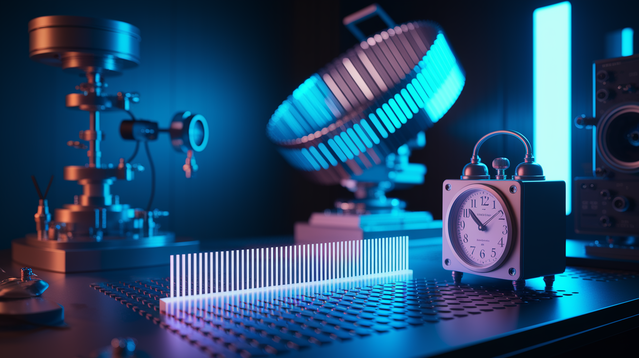
High precision Doppler spectroscopy turns tiny wavelength shifts into velocity measurements. Shifts so small they reveal planets orbiting distant stars. To detect an Earth mass planet in a year long orbit around a Sun like star, you need to measure velocity changes of about 10 centimeters per second. Walking speed. Laser frequency combs make that possible by giving you a ruler made of light, with tick marks spaced evenly and locked tightly to atomic time so every measurement references the same fundamental standard.
A laser frequency comb is a series of perfectly equally spaced spectral lines. Each one a precise frequency that can be traced back to a cesium atomic clock. When you send comb light through a spectrograph, those lines land on the detector at known positions. Any shift in those positions over time tells you exactly how the instrument drifted, mechanically, thermally, or optically, independent of the star you’re observing. You calibrate out the instrument, leaving only the star’s real motion.
Older calibration sources like thorium argon (ThAr) hollow cathode lamps produce emission lines scattered unevenly across the spectrum. Some wavelength regions are crowded, others nearly empty. The lines themselves are broad and asymmetric, shaped by collisions and electric fields inside the lamp. Worse, lamps age. Gas pressure changes, electrode surfaces degrade, and line intensities drift. A ThAr lamp might give you meter per second precision on a good night, but it won’t hold that precision across weeks or months. Laser frequency combs don’t age that way. The line spacing is set by the laser’s pulse repetition rate, a radio frequency you lock to an atomic standard. Coverage is uniform, limited only by how broadly you can spread the comb spectrum, and every line is narrow, symmetric, and stable.
When you’re hunting planets smaller than Neptune, especially rocky worlds in temperate orbits, you cross a threshold where instrument systematics become louder than the signal. A 10 cm/s velocity amplitude corresponds to a Doppler shift of about 200 hertz at visible wavelengths, roughly one part in a trillion. Calibration uncertainty at that level demands not just good reference lines, but traceable, reproducible reference lines that don’t introduce their own drifts. Frequency combs meet that standard because they are, fundamentally, optical representations of microwave time standards. The same atomic clock discipline that keeps GPS satellites synchronized keeps every comb tooth locked in place.
Physical Principles Behind Laser Frequency Comb Generation
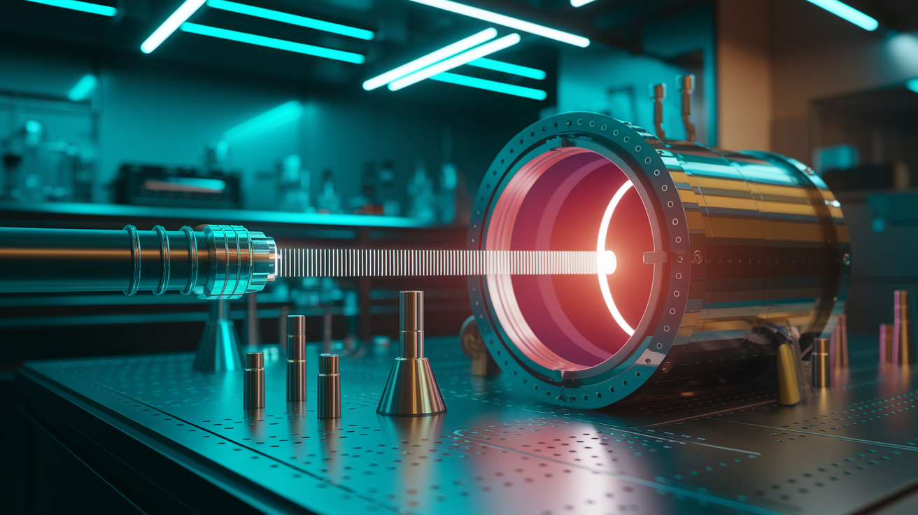
A frequency comb starts with a mode locked laser. A laser that produces ultrashort pulses instead of continuous light. Inside the laser cavity, light bounces back and forth between mirrors. Mode locking forces all the longitudinal modes (the standing wave patterns that fit inside the cavity) to oscillate in phase with one another. When they add up constructively, you get a brief, intense pulse of light. When they spread out again, the intensity drops. The laser emits a regular train of these pulses, like a strobe light with femtosecond flashes.
Each pulse in the train is a short burst in time, which means it’s broad in frequency. When you look at the spectrum, you see not one color but thousands of discrete optical frequencies, all evenly spaced. The spacing between adjacent frequencies equals the pulse repetition rate. How many pulses per second the laser produces. A laser running at 1 gigahertz repetition rate puts out one billion pulses per second, and its spectrum shows lines separated by 1 GHz. A 100 MHz laser has lines ten times closer together. The comb “teeth” are these discrete frequencies, and they span the full bandwidth of the pulse.
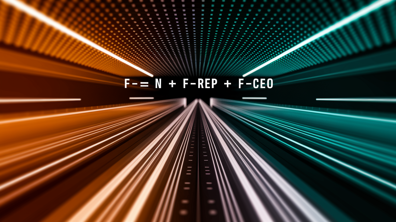
The spectrum isn’t just any collection of lines. It has a precise mathematical structure. Each tooth sits at a frequency given by f = n × frep + fCEO, where n is a large integer (the mode number), frep is the repetition rate, and fCEO is the carrier envelope offset frequency. The offset arises because the pulse envelope and the carrier wave inside it can slip relative to each other as the pulse circulates in the cavity. If you don’t control that slip, the whole comb drifts. Stabilizing both frep and fCEO locks every tooth to an absolute frequency reference, typically a GPS disciplined rubidium or cesium clock.
Stabilization mechanisms include:
Repetition rate locking. An electronic feedback loop compares the pulse train to a stable microwave oscillator and adjusts cavity length (often with a piezo mounted mirror) to keep f_rep fixed.
Carrier envelope offset control. A fraction of the comb spectrum is frequency doubled or otherwise processed to create a beat note that reveals f_CEO. That beat note is phase locked to a reference, stabilizing the offset.
Thermal management. Temperature changes alter cavity length and refractive index inside laser components. Active temperature control (often millikelvin level stability) and thermally insulating enclosures keep drift slow enough for the feedback loops to track.
Dispersion compensation. Intracavity dispersion affects pulse width and timing. Prism pairs, chirped mirrors, or dispersion compensating fiber keep pulses short and mode locking stable, which in turn keeps the comb structure clean.
Once both degrees of freedom are locked, every comb line becomes a known optical frequency, traceable to the primary time standard. When you route that light into a spectrograph, you’re effectively projecting a grid of atomic clock referenced markers onto your detector. Any wavelength calibration you derive from that grid inherits the clock’s long term accuracy and short term stability, translating directly into Doppler velocity precision at the centimeter per second level if systematics in the spectrograph itself are controlled.
Integrating Laser Frequency Combs Into High‑Resolution Spectrographs
Getting comb light into a working astronomical spectrograph means solving several optical and engineering challenges. The comb output is typically a collimated free space beam at infrared wavelengths (often around 1550 nanometers for telecom grade fiber lasers). You need to couple that into single mode fiber, broaden the spectrum to cover visible or near infrared windows where your spectrograph operates, flatten the intensity envelope so all lines have similar brightness, and match the comb’s line spacing to the instrument’s resolving power. Each step adds complexity, but each is necessary to turn a lab laser into an observatory calibration source.
Fiber coupling starts with mode matching optics that focus the comb beam into a single mode fiber core, typically a few micrometers wide. Alignment is sensitive. Microradians of tilt or microns of lateral offset cut coupling efficiency. Once in fiber, you can send the light through nonlinear broadening stages. A common approach uses highly nonlinear fiber (HNLF), where the intense comb pulses undergo self phase modulation and four wave mixing, spreading the spectrum from a narrow telecom band into hundreds of nanometers. You might follow HNLF with additional amplification and second stage broadening, or with frequency doubling in a nonlinear crystal, to reach blue and green wavelengths. The goal is continuous coverage across the spectrograph’s bandpass, or at least dense enough sampling that calibration fits don’t leave big gaps.
Spectral flattening addresses the problem that broadened combs rarely have uniform power per line. The envelope might peak in the red and drop sharply in the blue, leaving some lines too faint to use and others saturating the detector. Filtering cavities (Fabry Pérot etalons with free spectral ranges chosen to transmit every Nth comb line) can reshape the envelope by selecting subsets of lines and suppressing others. You can also use shaped gain media or amplitude modulators, though those add loss and complexity. The trade is between coverage and uniformity. A flatter spectrum simplifies calibration algorithms but may sacrifice total throughput.
Matching comb spacing to spectrograph resolution is about avoiding ambiguity. If the comb’s repetition rate is too low, adjacent lines land on the same resolution element and you can’t tell them apart. If it’s too high, you get one line per many pixels, wasting information. An ideal match puts several comb lines within each resolution element of the spectrograph, giving you well sampled line profiles you can centroid accurately. For a spectrograph with resolving power R around 100,000 at 500 nm (line width roughly 1.5 GHz), a comb repetition rate near 10 to 25 GHz works well. Building and stabilizing such high repetition rate “astrocombs” is harder than maintaining gigahertz class systems, so many current implementations accept coarser sampling or use filtering tricks to avoid the problem.
Calibration Procedures Using Laser Frequency Combs
The calibration workflow wraps the science observation in reference exposures that map the spectrograph’s wavelength solution and track any drifts. You start the night by taking a comb spectrum with the same exposure settings you’ll use for stars. Same detector readout mode, same binning, same slit or fiber configuration. That first spectrum establishes a baseline pixel to wavelength mapping across every order and every region of the detector.
The full sequence typically follows these steps:
Initial reference exposure. Record a comb spectrum at the beginning of the observing session, ensuring all stabilization locks (repetition rate, CEO, thermal control) have settled and the comb output is stable.
Wavelength solution fit. Extract line positions from the reference spectrum, assign known frequencies to each detected line (using the comb equation f = n × frep + fCEO and integer mode numbers determined from approximate wavelength), and fit a polynomial or spline model mapping pixel coordinate to frequency.
Pre science calibration. Just before the target star exposure, take a short comb frame to capture the instrument state at that moment. Any thermal drift or mechanical settling that occurred since the initial reference.
Post science calibration. Immediately after the star exposure, record another comb frame. Compare line positions to the pre science frame. Pixel shifts here reveal drift during the science integration.
Nightly and long term tracking. Repeat the previous two steps around every science exposure. At the end of the night, compare the final comb spectrum to the initial reference. Over weeks and months, archive all calibration frames to model slow drifts (seasonal temperature cycles, aging optics, detector charge transfer effects) and refine the wavelength solution retrospectively.
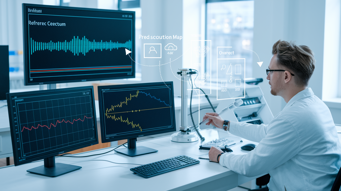
Processing these calibration frames into velocity corrections involves centroiding each comb line (usually Gaussian or Voigt profile fits), calculating pixel shifts relative to the reference, converting shifts to wavelength offsets using the local dispersion (angstroms per pixel or hertz per pixel), and finally translating wavelength offsets into velocity via the Doppler formula v/c = Δλ/λ. Modern pipelines cross correlate entire comb spectra against templates or use maximum likelihood fits that account for detector noise and line blending. The output is a time series of instrument velocity zero points. Corrections you subtract from the raw stellar radial velocities to remove spectrograph drift and leave only the star’s real motion.
Instrumental Error Sources and Stability Considerations
Even with a perfect frequency comb, the spectrograph itself introduces errors. Temperature changes shift optical elements, altering focal lengths and grating angles. A millikelvin drift in the detector’s CCD temperature can move charge transfer efficiency and change the apparent centroid of every line. Atmospheric pressure variations flex vacuum chamber windows or change the refractive index of air paths if the instrument isn’t fully evacuated. Mechanical vibrations from telescope drives, cooler pumps, or even wind shake on the dome nudge mirrors and fibers. Each of these effects shows up as a spurious velocity signal unless you measure and correct it.
Combs help because they experience the same instrumental drifts the starlight does. When the grating tilts slightly due to thermal expansion, both the star’s spectral lines and the comb lines shift together. Subtracting the comb measured shift cancels the effect. Where combs fall short is when the error source affects starlight and calibration light differently. If, for example, the star’s light path and the comb’s injection point see different thermal environments, or if illumination non uniformity on the detector (flat field errors) varies between the two sources. Simultaneous calibration setups, where comb light and starlight share the same fiber or slit and traverse identical optics, minimize this differential error.
Detector non uniformity is subtle but important at centimeter per second precision. Pixel to pixel sensitivity variations, charge transfer inefficiency in CCDs, and persistence (charge left over from previous exposures) all distort line profiles. A comb line might land on a cluster of hot pixels one night and cold pixels another, shifting its measured centroid even though the true wavelength didn’t change. Regular flat fielding helps, but high frequency sensitivity structure requires dense calibration sampling (many comb lines per order) to map and correct. Infrared detectors add read noise and dark current. You trade longer exposures for better signal to noise, but longer exposures accumulate more drift, so you optimize integration time and calibration cadence together.
Stability strategies that work in practice include:
Vacuum or pressure stabilized enclosures. Sealing the spectrograph in a vacuum tank eliminates air path refraction changes and reduces convective temperature gradients. Pressure control to the millibar level offers a cheaper alternative for some designs.
Active temperature regulation. Multi zone thermal control, often with millikelvin setpoint stability, keeps optical benches, gratings, and cameras isothermal. Some systems add glycol cooled enclosures or multi layer insulation blankets around sensitive components.
Continuous drift tracking. Recording comb spectra every few minutes, or even continuously via a separate calibration fiber, lets you interpolate instrument zero point between science exposures rather than assuming it holds constant over an hour long integration.
Real‑World Deployments and Performance Achievements
Laser frequency combs have moved from proof of concept demonstrations to operational calibration systems on some of the world’s leading exoplanet spectrographs. Early work in the late 2000s showed that near infrared combs could deliver wavelength calibration equivalent to about 9 meters per second Doppler precision, already better than ThAr lamps, but still far from the centimeter per second goal. Subsequent improvements in spectral coverage, line filtering, and simultaneous reference techniques have pushed performance into the sub meter per second regime on multiple instruments.
HARPS N, the high resolution spectrograph on the Telescopio Nazionale Galileo in the Canary Islands, was an early adopter. Comb integration there involved a green extended astrocomb covering roughly 500 to 620 nanometers with a repetition rate near 18 GHz, giving about 30,000 lines across the bandpass. Simultaneous ThAr and comb calibration tests in the mid 2010s demonstrated that the comb reduced long term systematic drifts and improved night to night velocity zero point stability to around 10 centimeters per second, a factor of several better than lamps alone. That stability opened the door to detecting lower amplitude signals and refining orbits of known planets with higher confidence.
ESPRESSO, the Echelle SPectrograph for Rocky Exoplanets and Stable Spectroscopic Observations at the Very Large Telescope, was designed from the start with extreme stability in mind. A thermally controlled, vacuum enclosed optical bench and both a Fabry Pérot etalon and a laser frequency comb for calibration. The ESPRESSO comb is a visible wavelength astrocomb with repetition rate around 18 GHz, filtered and spectrally flattened to provide uniform coverage from 380 to 780 nanometers. Published results show the instrument achieving radial velocity precision around 10 centimeters per second on bright stars over timescales of months, with the comb enabling correction of complex, time varying instrumental signatures that etalons alone couldn’t fully capture.
| Instrument | Achieved Precision | Notes |
|---|---|---|
| HARPS‑N (TNG) | ~10 cm/s (long‑term) | 18 GHz visible astrocomb; simultaneous calibration fiber; operational since mid‑2010s |
| ESPRESSO (VLT) | ~10 cm/s (months) | 18 GHz visible comb + Fabry‑Pérot; vacuum enclosure; designed for sub‑m/s RV |
| EXPRES (Lowell) | ~30 cm/s (demonstrated) | Green astrocomb; environmental control; focus on bright‑star high‑cadence observations |
| NEID (WIYN) | ~27 cm/s (on‑sky) | Etalon + LFC hybrid; port at Kitt Peak; targets solar‑type stars for Earth‑mass planets |
| HPF (HET) | Sub‑m/s (near‑IR) | Near‑infrared comb (0.8–1.3 µm); tailored for M‑dwarf planet searches; thermally stabilized |
EXPRES, the EXtreme PREcision Spectrograph at the Lowell Discovery Telescope, integrates a green wavelength astrocomb and targets 30 centimeters per second single measurement precision on bright stars. The system uses a mode filtered comb at approximately 10 GHz repetition rate, environmental isolation (temperature and pressure stabilization), and a simultaneous solar/stellar calibration channel. Early on sky results confirmed sub meter per second internal precision, with systematic error budgets showing that most residual scatter comes from stellar activity (spot driven line profile changes) rather than instrumental drift. A validation that the calibration system is working as designed.
NEID, the NN EXPLORE Exoplanet Investigations with Doppler spectroscopy instrument on the WIYN telescope at Kitt Peak, uses a hybrid approach. A Fabry Pérot etalon for dense wavelength coverage and a laser frequency comb for absolute referencing. The comb operates near 25 GHz repetition rate across 380 to 930 nanometers, locked to GPS disciplined rubidium. Commissioning data in 2020 to 2021 showed on sky radial velocity precision around 27 centimeters per second on solar type stars, with systematic trends tracked and removed using the comb’s nightly drift measurements. This performance puts Earth mass planets in habitable zones within reach for multi year monitoring campaigns.
Final Words
In the action, we showed how laser frequency combs give the dense, stable reference lines that push Doppler precision to cm/s, why the comb physics matters, and how careful coupling and calibration turn that stability into usable measurements.
We ran through the practical workflow, the main instrumental error sources, and real deployments that proved the method on sky.
Bottom line: calibrating high-resolution spectrographs with laser frequency combs for Doppler measurements makes tiny stellar wobbles trackable, and that gives us a clearer path to finding small planets.
FAQ
Q: Why are laser frequency combs essential for cm/s radial velocity calibration?
A: Laser frequency combs are essential because they provide a dense, stable set of reference lines (a ruler of equally spaced laser lines) that let us measure tiny Doppler shifts with cm/s accuracy.
Q: How do laser frequency combs unlock cm/s Doppler precision?
A: Laser frequency combs unlock cm/s precision by giving uniform, well‑known lines across the spectrum, so pixel shifts map directly to velocity and tiny instrument drifts are measured and removed precisely.
Q: How do laser frequency combs compare to ThAr lamps for calibration?
A: Laser frequency combs outperform ThAr lamps by offering long‑term stability, dense uniform line spacing, and wide wavelength coverage, while ThAr lines are sparse, uneven, and suffer from aging and lamp variability.
Q: How are laser frequency combs generated and stabilized?
A: Laser frequency combs are generated by mode‑locked lasers producing pulse trains whose spectrum shows evenly spaced modes; stabilization locks the repetition rate and the carrier‑envelope offset (CEO) to keep line positions fixed over time.
Q: How are frequency combs integrated into high‑resolution spectrographs?
A: Frequency combs are integrated via fiber coupling, filtering cavities, and spectral flattening so line spacing matches the spectrograph resolution and the comb illuminates the detector evenly and stably.
Q: What are the typical calibration procedures using a laser frequency comb?
A: Typical calibration procedures record comb spectra before and after science exposures, map comb lines to detector pixels, track instrument drift, and convert pixel shifts into velocity corrections during data processing.
Q: What instrumental error sources do combs help correct?
A: Laser frequency combs help correct temperature and pressure changes, mechanical flexure, and detector non‑uniformity by continuously monitoring spectral line positions and enabling precise drift compensation.
Q: What real‑world performance have combs achieved on spectrographs?
A: In practice, combs on instruments like HARPS, HARPS‑N, EXPRES, and ESPRESSO have pushed from sub‑m/s down toward cm/s precision, improving long‑term stability and drift correction for precise radial velocities.
Q: What does frequency comb calibration mean for exoplanet detection limits?
A: Frequency comb calibration lowers the instrumental noise floor, letting us detect smaller radial velocity signals—closer to Earth‑mass planets—though stellar activity and noise still set practical detection limits.