
Which matters more in astronomy: how bright an object is, or what its light tells us about composition and motion?
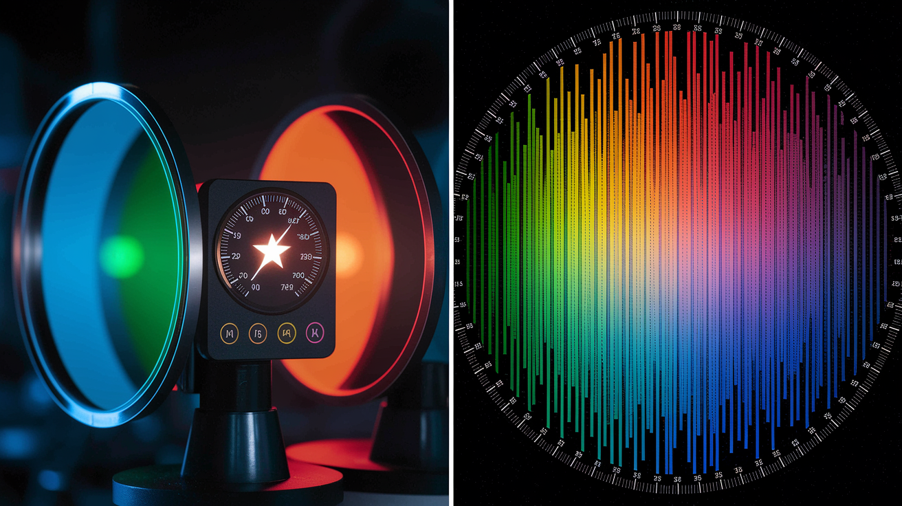
Photometry measures brightness across broad color bands.
It’s like a light meter giving a single number.
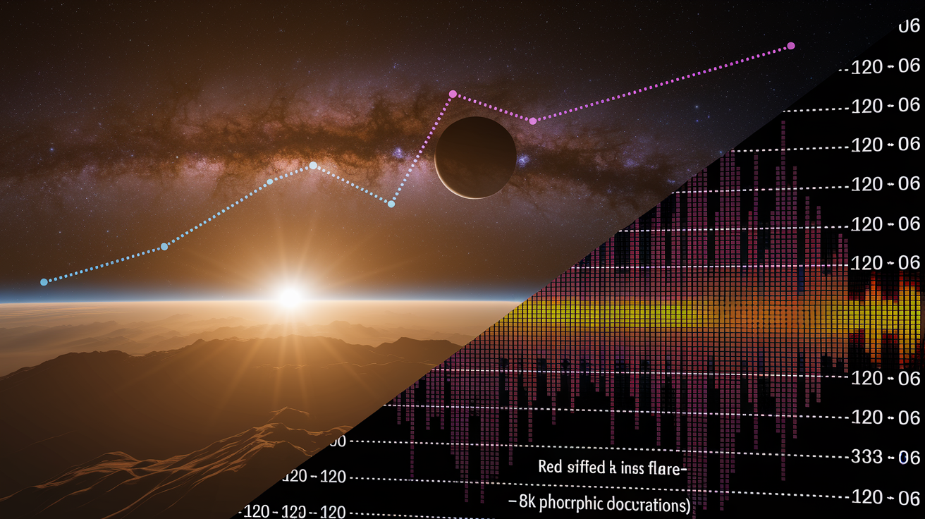
Spectroscopy splits light into a spectrum (a rainbow of wavelengths) and reads fingerprints, like elements, temperature, and Doppler shifts.
Photometry is fast, great for surveys and time-series.
Spectroscopy is slower but shows composition and motion.
This post shows the core difference, when to use each, and why they work together to turn a bright dot into a real story.
Core Differences Between Photometry and Spectroscopy in Astronomy
Photometry tells you how bright something is across one or more broad color bands. It’s measuring total light, filtered through blue, green, or red glass. You get a single number: magnitude, flux, or a point on a light curve. Spectroscopy splits that same light into hundreds or thousands of narrow slices, like spreading sunlight into a rainbow. Instead of one brightness reading, you’re looking at a graph showing intensity at every specific wavelength. And that graph carries fingerprints. Absorption lines, emission lines, the chemical makeup of a star, its temperature, whether it’s racing toward you or away.
Photometry can’t tell you what something’s made of or how fast it’s moving. It sees brightness changes but can’t distinguish whether a star dimmed because it cooled, because dust drifted in front, or because a companion blocked it. Spectroscopy answers those questions. It shows which elements are there and how Doppler shifts move known lines. A hydrogen line normally at 656.3 nm shifted to 656.4 nm? The object’s receding at roughly 140 km/s. But spectroscopy is slow. You’re spreading every photon across many detector pixels, so you need much longer exposures or a much bigger telescope to hit the same signal quality as photometry on the same target.
Astronomers pick photometry when time matters, when they’re covering huge patches of sky, or when they’re hunting faint objects in bulk. A single image can measure thousands of stars in seconds. They pick spectroscopy when they need to know what something is, not just how bright. Classifying a supernova, measuring a star’s metal content, confirming an exoplanet’s orbital speed? You need a spectrum. Often the two work together. Photometry finds the candidates. Spectroscopy explains what they are.
| Method | What It Measures |
|---|---|
| Photometry – Brightness | Total flux in one or more broad bands; outputs magnitudes, colors, light curves |
| Spectroscopy – Wavelength Detail | Flux versus wavelength; outputs spectral lines, velocities, composition |
| Photometry – Outputs | Numerical brightness, color indices, time-series light curves |
| Spectroscopy – Time Demands | 10× to 100× longer exposure per target for comparable signal-to-noise |
| Typical Applications | Photometry: variable-star monitoring, transit detection, supernova discovery. Spectroscopy: redshifts, abundances, radial velocities |
Understanding Photometry Methods Used in Astronomy
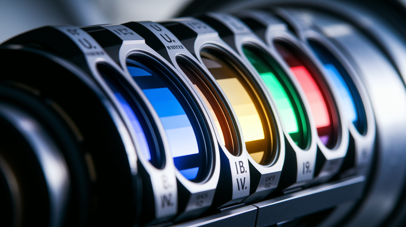
Photometric measurements lean on filters that decide which wavelengths hit the detector. Standard systems like Johnson–Cousins use filters labeled U (ultraviolet), B (blue), V (visual green), R (red), I (infrared). Each filter spans roughly 100 to 1,000 Ångströms (10 to 100 nanometers), wide enough to grab plenty of photons but narrow enough to separate colors. Johnson V is the most popular for amateurs because it matches how the human eye sees and lines up with historical magnitude scales. Compare brightness in two or more filters and you get a color index like B–V, which hints at temperature. Hot stars look blue (negative B–V), cool stars look red (positive B–V). A single filter gives you one data point. Multiple filters start to sketch the object’s spectral energy distribution, though it’s still just a handful of broad samples.
CCDs and CMOS sensors respond linearly to light across most of their range. Double the photons, double the signal. That linearity is what makes photometry quantitative. But every sensor hits a ceiling. Too many photons on a pixel and charge spills into neighbors, creating streaks called blooming. Anti-blooming gates can stop the spill but also shorten the detector’s useful range, so you’ve got to plan exposures carefully. Before you measure anything, images need calibration. Bias frames (electronic offset), dark frames (thermal noise), flat-field frames (pixel-to-pixel sensitivity variations). Without that work, a 1 percent brightness change can hide inside 5 percent instrumental noise.
Three photometry modes boost accuracy in different ways. Aperture photometry draws a circle around the star, adds up all the pixel counts inside, then subtracts background measured in a surrounding ring. You have to use the same aperture size for the target and comparison stars or systematic errors creep in. PSF photometry fits a model of the star’s point-spread function to every source in a crowded field, teasing apart overlapping profiles. Differential photometry divides the target’s brightness by one or more comparison stars in the same frame, canceling atmospheric extinction and most instrumental drift. On a good night from the ground, differential photometry can hit 1 to 10 millimagnitudes precision (0.001 to 0.01 mag). From space, missions like Kepler and TESS routinely reach 20 parts per million (0.00002 mag) for bright stars. Enough to spot an Earth-size planet crossing a Sun-like star.
Photometry’s real strength shows up in light curves and time-domain surveys. Variable stars reveal periods and amplitudes. Eclipsing binaries trace eclipse depths and durations. Exoplanet transits appear as tiny, repeatable dips. 1 percent for a hot Jupiter, 0.01 percent for an Earth analog. Supernova hunters image the same galaxies night after night, subtract old images from new ones, flag anything that brightens. In June 2015, amateurs with telescopes 200 mm or larger recorded rapid visible-light flickering from V404 Cygni, a black-hole binary. That high-speed photometry, sampling brightness every few seconds, captured optical output from the accretion disk for the first time in the visible band.
How Astronomical Spectroscopy Reveals Physical Properties of Objects
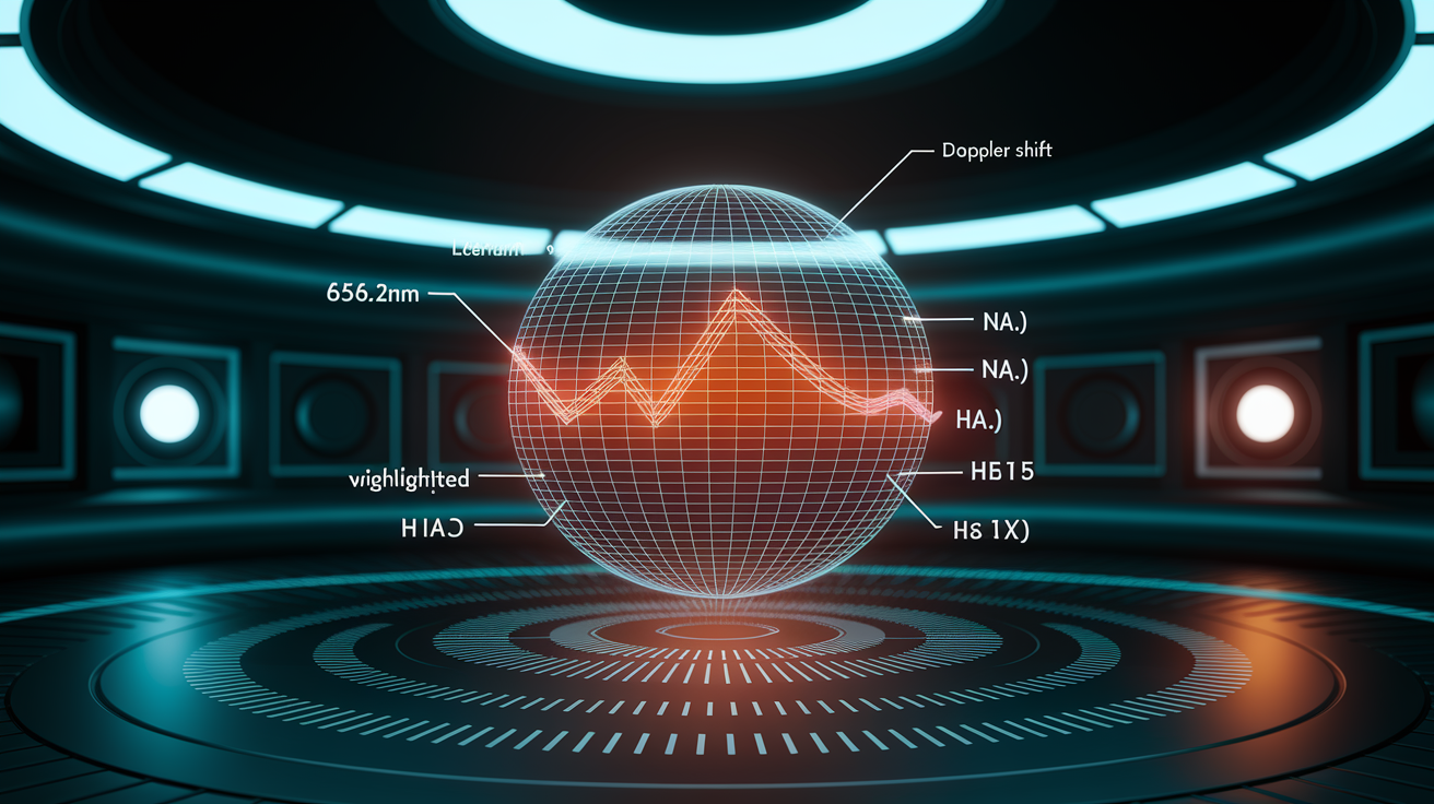
A spectrum is light sorted by wavelength. Every atom or molecule stamps a signature pattern of dark absorption lines or bright emission lines at specific spots in that rainbow. Hydrogen always absorbs at 656.3 nm (the red Hα line), 486.1 nm (blue Hβ), and so on. Sodium vapor lamps spit out a tight yellow doublet near 589 nm. When you see those lines in a star’s spectrum, you know hydrogen and sodium are hanging out in the outer layers. The relative strength of different lines tells you temperature. Hot stars ionize metals and show helium lines. Cool stars show molecular bands from titanium oxide or water. Line profiles also encode physics. A broad, smooth profile? The star’s spinning fast or has turbulent motions. A sharp, narrow line suggests a calm photosphere. Double-peaked emission often means a rotating disk seen edge-on.
Spectral resolution, written as resolving power R = λ / Δλ, decides how much detail you can see. Low-resolution spectra (R ≈ 100 to 1,000) blur neighboring lines together but collect light quickly. Useful for classifying objects or grabbing crude redshifts. Medium resolution (R ≈ 1,000 to 10,000) separates most strong lines and starts to show velocity structure. High resolution (R ≈ 20,000 to 100,000 or more) splits fine details like isotope shifts and measures Doppler velocities down to about 1 meter per second or better. Earth’s orbital motion around the Sun shifts stellar lines by ±30 km/s over six months, so even modest resolution can measure that. Detecting a Jupiter-mass planet’s reflex tug (tens of meters per second) needs R above 50,000 and obsessive wavelength calibration.
Real instruments range from simple to complex. A £200 Star Analyser transmission grating slides into a 1.25-inch eyepiece holder, works with DSLRs or cooled cameras, delivers R ≈ 100 to 200. Software like RSpec can measure line positions and rough equivalent widths. Enough for learning or bright emission-line targets. At the other end, the Shelyak ES0002-Lhires III echelle spectrograph costs significantly more and needs precise guiding, but it hits R ≈ 15,000 to 20,000, resolving velocity shifts and fine chemical details. Every spectrograph needs wavelength calibration. Usually an arc lamp with known emission lines (neon, argon, thorium) recorded before or after the target. The calibration frame maps detector pixels to nanometers so you know exactly where each stellar line sits.
Equipment Differences Between Photometry and Spectroscopy Systems
Photometry uses the same imaging cameras as regular astrophotography. CCD or CMOS sensors cooled to cut thermal noise, paired with filter wheels holding Johnson–Cousins, SDSS ugriz, or custom narrowband sets. The light path is simple. Telescope, optional focal reducer, filter, detector. The pixel scale can be matched to the seeing disk for efficient photon collection. Data reduction is straightforward. Subtract bias and dark frames, divide by a normalized flat field, measure star positions via plate-solving, run aperture or PSF photometry in software like Maxim DL, AstroImageJ, or IRAF. Calibration is quick because most frames are reusable across a night or even longer if the camera setup doesn’t change.
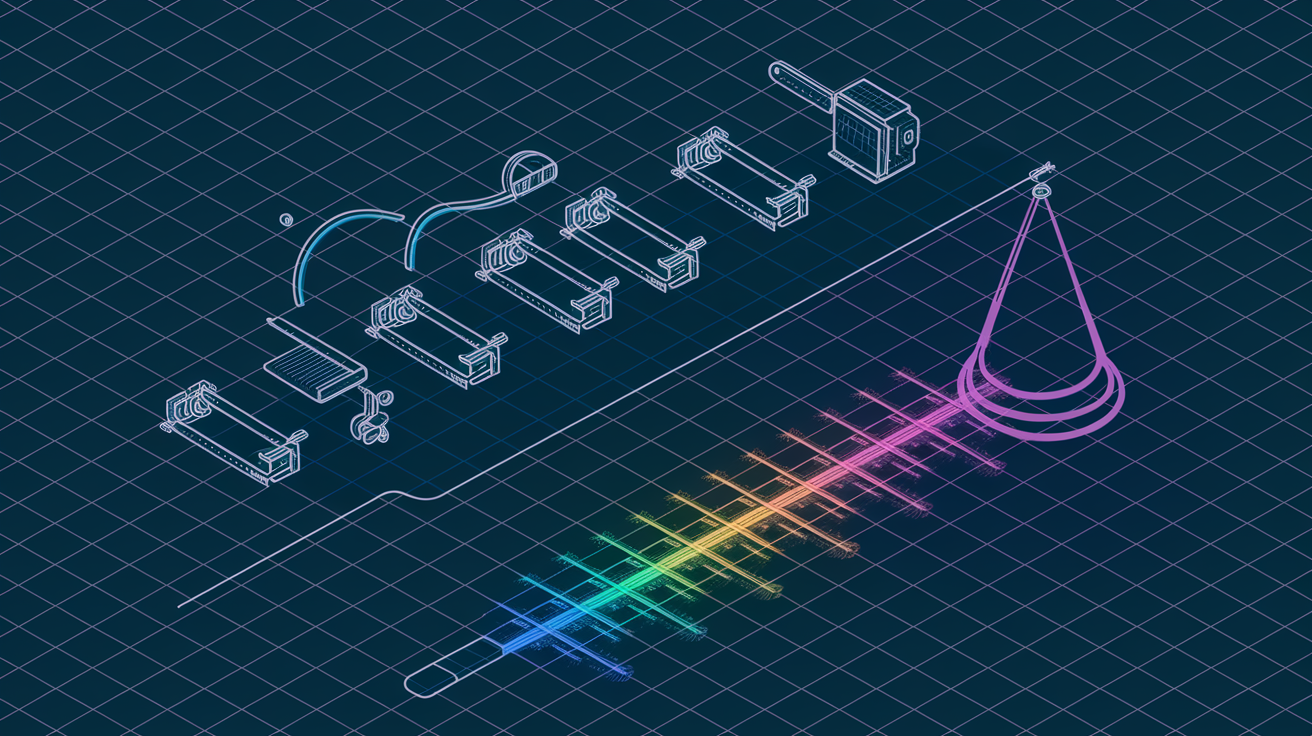
Spectroscopy adds several layers of complexity.
Dispersive element: A grating or prism spreads light into a spectrum, replacing the simple filter. Echelle designs cross-disperse onto a 2D grid for high resolution.
Slit or fiber input: A narrow slit isolates the target and defines spectral resolution. Fiber-fed systems can multiplex dozens of objects but add alignment challenges.
Wavelength calibration: Arc lamps, hollow-cathode sources, or laser frequency combs provide reference lines. Calibration must be repeated if temperature drifts or the instrument flexes.
Longer exposures: Photons are divided among hundreds of wavelength bins instead of summed in one broad filter, so reaching the same signal-to-noise per resolution element typically takes 10× to 100× more time.
A high-precision radial-velocity spectrograph also needs an ultra-stable optical bench, sometimes temperature-controlled to millikelvin stability, and simultaneous calibration (a second fiber feeding the calibration source into the spectrograph at the same time as the starlight). Photometry can run all night unattended with a sequencer. Spectroscopy often needs manual target acquisition, guiding checks, iterative focus adjustments. Any defocus smears the spectrum and ruins resolution.
Practical Applications: When Photometry or Spectroscopy Is the Right Tool
Photometry wins when you want to watch something change or survey large areas quickly. Exoplanet transits are pure photometry. Measure the star’s brightness every few minutes, catch the 0.01 to 1 percent dip when the planet crosses the disk, repeat to confirm the period. Ground-based projects and space missions like Kepler, TESS, PLATO have found thousands of planets this way. Variable-star monitoring is another photometry workhorse. Cepheids, RR Lyrae, Mira variables, eclipsing binaries all show periodic or irregular brightness changes that reveal pulsation physics, binary orbits, distances. The Cepheid period-luminosity relation, discovered around 1912 by Henrietta Leavitt, turned photometry into a cosmic yardstick still used today to calibrate the distance ladder.
Spectroscopy steps in when you need to know what something is or how it moves. Supernova hunters use photometry to find the explosion. Spectroscopy classifies the type. Type Ia supernovae (white-dwarf thermonuclear detonations) show no hydrogen lines and a strong silicon feature. Type II (core-collapse of massive stars) show hydrogen. Knowing the type lets you interpret the light curve and use Type Ia events as standardizable candles. In the late 1990s, two teams combined supernova photometry (measuring peak brightness and decline rate) with spectroscopy (confirming type and measuring redshift) to discover that cosmic expansion is accelerating. Work that earned the 2011 Nobel Prize. Radial-velocity exoplanet detection is all spectroscopy. Measure the star’s Doppler wobble induced by an orbiting planet, reaching precision around 1 m/s for state-of-the-art instruments. A hot Jupiter tugs its star at tens of meters per second. An Earth-mass planet in a one-year orbit induces about 0.1 m/s, right at the bleeding edge of current capability.
Combined-method campaigns are now standard. Wide-field photometric surveys (Pan-STARRS, Zwicky Transient Facility, Vera Rubin Observatory) scan the sky nightly, flagging anything that moves or changes. Spectroscopic follow-up from 8 to 10 meter telescopes then provides redshifts, abundances, velocity fields. Epsilon Aurigae, a peculiar eclipsing binary with a 27-year period, saw its 2009 to 2011 eclipse monitored by amateur spectroscopists who recorded previously unmeasured variations in the spectrum of the eclipsing object, filling gaps left by professional schedules.
Five landmark examples across techniques:
Cepheid period-luminosity relation (≈1912): photometry established the distance scale
Cosmic acceleration discovery (1998): supernova photometry plus spectroscopic typing and redshifts
First exoplanet radial-velocity detection (51 Peg b, 1995): high-resolution spectroscopy, ~50 m/s amplitude
Kepler exoplanet transits (2009 to 2018): space-based photometry, ~20 ppm precision, thousands of planets
V404 Cygni optical flickering (June 2015): high-speed photometry by amateurs, ≥200 mm apertures, accretion-disk physics
Performance Limits: Exposure Time, SNR, and Observing Constraints
Signal-to-noise ratio (SNR) controls what you can detect and how precisely you can measure it. SNR scales roughly as the square root of the number of photons collected, so quadrupling your exposure time or aperture area doubles SNR. Photometry collects all photons across a filter’s bandpass into one measurement, so reaching SNR = 100 on a moderately bright star might take 10 to 60 seconds from the ground. Spectroscopy divides those same photons among 500 or 5,000 wavelength bins, so each bin gets far fewer counts. To reach SNR = 100 per resolution element at R = 10,000 typically needs 10× to 100× longer exposures than an equivalent photometric measurement, depending on the target’s brightness and the instrument’s throughput. Faint targets or very high resolution push exposure times to hours, even on large telescopes.
Practical limits come from sky background, atmospheric extinction, saturation. Photometry must subtract the diffuse glow of the sky (moonlight, airglow, light pollution) measured in the aperture’s background annulus. Bright sky raises the noise floor and limits how faint you can go in a given exposure. Spectroscopy faces the same sky background spread across every wavelength bin, plus telluric absorption. Water vapor and oxygen in Earth’s atmosphere carve hundreds of lines into infrared and red spectra that must be removed by dividing out a standard-star observation or atmospheric model. Extinction correction accounts for how much starlight the atmosphere absorbs as a function of airmass. Photometry uses extinction coefficients per filter. Spectroscopy must correct the entire spectral shape. Saturation is easier to avoid in photometry (just shorten the exposure), but a saturated spectral line loses all velocity and abundance information because the peak is clipped.
| Limitation | Photometry | Spectroscopy |
|---|---|---|
| Exposure Time | Seconds to minutes for bright/moderate targets | Minutes to hours; 10×–100× longer per SNR unit |
| Sky Background | Subtracted via annulus; limits faint-object depth | Subtracted per wavelength; telluric lines complicate IR/red |
| Saturation Risk | Easily managed by shorter exposures | Ruins line profiles; requires careful exposure planning |
Combining Photometry and Spectroscopy in Modern Astronomy
Almost every major discovery in time-domain and survey astronomy now uses both methods in sequence. Photometric surveys like the Zwicky Transient Facility image the entire northern sky every few nights, flagging supernovae, asteroids, variable stars, transient events. Those candidates then feed into a spectroscopic queue on 2 to 10 meter telescopes that confirm the nature of each object, measure redshift, classify supernova type, check for unusual spectral features. Photometric redshifts, estimated by fitting an object’s brightness across multiple filters to template spectral energy distributions, give rough distance estimates for millions of galaxies. Spectroscopic redshifts, measured from individual emission or absorption lines, provide precision to better than 0.001 in redshift and anchor the photometric calibration.
Exoplanet science relies on the synergy even more. Transit photometry finds planets and measures their radius (from the depth of the dip and the star’s known size). Radial-velocity spectroscopy measures the planet’s mass (from the amplitude of the Doppler wobble and the orbital period). Combine radius and mass, and you get mean density. The first step toward understanding composition. Neither method alone delivers that. The 1998 accelerating-universe result also depended on both. Photometric light curves determined each supernova’s peak brightness and decline rate (needed to standardize the candle), while spectroscopy confirmed it was Type Ia and measured the redshift (needed to place it in cosmic history).
Typical combined-use workflows:
Survey to follow-up: photometric all-sky patrol identifies candidates; spectroscopy provides physical classification and precise parameters
Target selection: photometry measures colors or variability; spectroscopy confirms interesting objects worth deeper study
Calibration anchors: spectroscopic standard stars calibrate photometric zero-points and color transformations
Population studies: photometry provides statistics for millions of sources; spectroscopy characterizes representative subsamples in detail
Final Words
We jumped straight into how the two methods differ: photometry measures total brightness and makes light curves, while spectroscopy spreads light to reveal spectral lines, chemistry, temperature, and motion.
You saw equipment, observing limits, and when each method wins: photometry is fast and great for surveys and transits, while spectroscopy gives physical detail but needs more photons and longer exposure.
So, if you’re choosing a setup or reading a paper, remembering the photometry vs spectroscopy difference for astronomy (brightness and timing versus wavelength-resolved physics) keeps things clear. Use both when you can. Happy observing.
FAQ
Q: What is the difference between photometry and spectroscopy?
A: The difference between photometry and spectroscopy is that photometry measures total brightness through filters to give magnitudes, colors, and light curves, while spectroscopy spreads light by wavelength to reveal composition, temperature, and velocity.
Q: Why is photometry important in astronomy?
A: Photometry is important in astronomy because it tracks brightness and its changes, enabling distance estimates, exoplanet transit detection, variable-star studies, and wide surveys that identify targets for deeper study.
Q: Do astronomers use spectroscopy for stars?
A: Astronomers use spectroscopy for stars to measure chemical composition, temperature, surface gravity, magnetic fields, and radial velocity, which drive classification, age estimates, and detection of binaries or orbiting planets.
Q: What is the difference between astrometry and photometry?
A: The difference between astrometry and photometry is astrometry measures precise sky positions and motions to map orbits, while photometry measures brightness and variability to study flux changes and physical behavior.