
What if I told you we can weigh unseen planets by measuring a star’s tiny wobble?
It works because starlight shifts when the star moves toward or away.
We read that shift in a spectrum (a light fingerprint), then convert the tiny wavelength change into a speed.
I’ll walk you step-by-step through the instruments, calibration options, reduction steps, and how to spot astrophysical and instrumental errors so you can trust the velocity you measure.
Core Principles Behind Measuring Radial Velocity
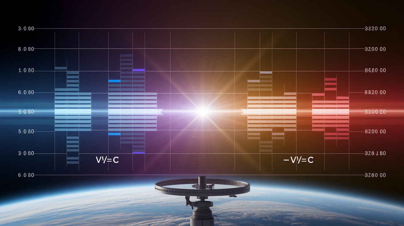
Radial velocity tells you how fast a star’s moving toward or away from Earth. You’ll usually see it in kilometers per second or meters per second. When a star races toward you, its wavelengths get compressed. Moving away? They stretch out. This isn’t some optical illusion. The wavelengths actually change because of relative motion.
The Doppler formula connects everything: Δλ/λ = v/c. Δλ is what you observe minus the rest wavelength, λ is the rest wavelength, v is the radial velocity, and c is light speed (about 300,000 km/s). Say you measure a spectral line at 656.5 nm that should sit at 656.3 nm in the lab. That 0.2 nm shift? Star’s moving away. Do the math: 0.2 divided by 656.3 gives roughly 0.0003, so v comes out around 90 km/s recession.
The whole method depends on comparing what you see with lab references. Stars make absorption lines at specific wavelengths tied to elements like hydrogen, calcium, iron. You identify which line you’re looking at, grab its known rest wavelength from atomic databases, measure where it actually lands in your spectrum, calculate the shift, then convert to velocity. Same star observed six months apart might show different velocities if it’s orbiting something or your own motion changed. But the core stays the same: measure, compare, apply the formula.
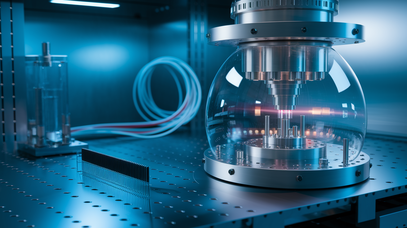
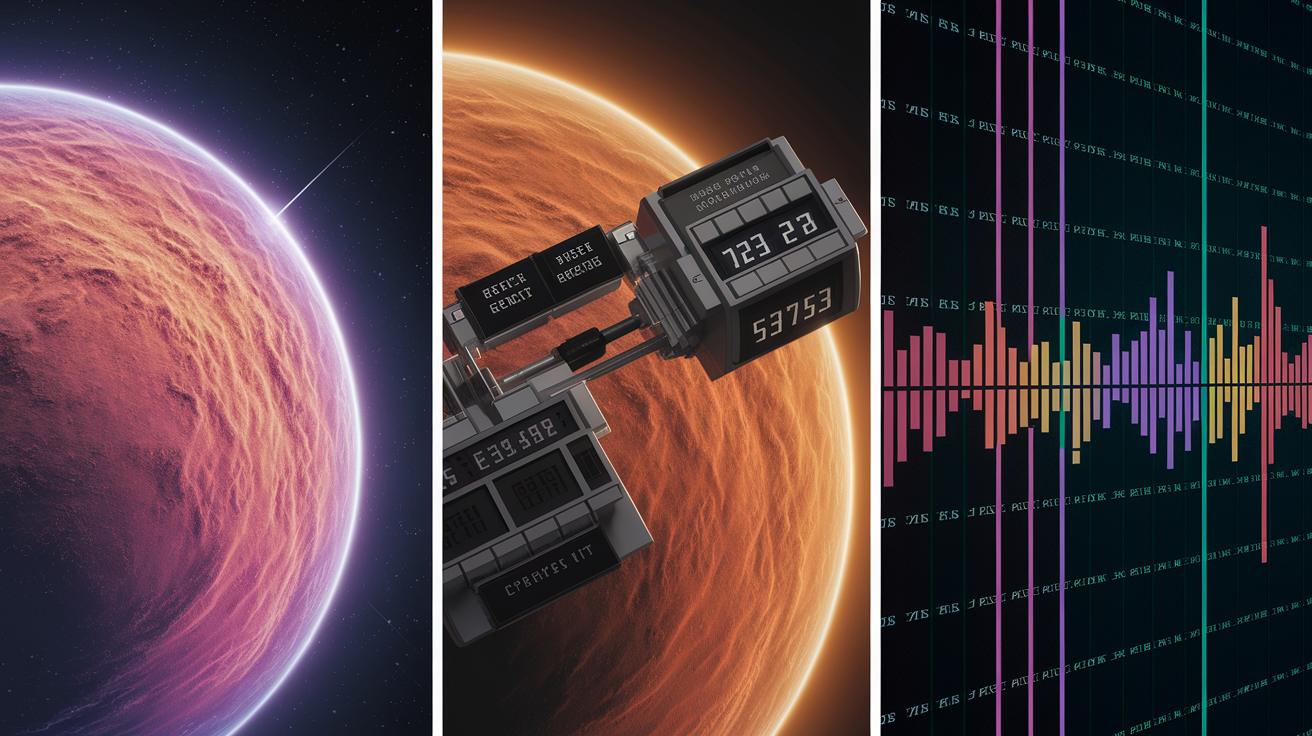
Instrumentation Required for Doppler Spectroscopy
Spectral resolution controls how finely you can separate wavelengths. It’s written as R, the ratio of wavelength to the smallest difference you can resolve. R of 50,000 means you can pull apart features 1/50,000 of a wavelength apart. Higher resolution spreads the spectrum across more pixels, so tiny shifts become easier to catch. Detecting exoplanet wobbles at a few meters per second? You need R above 50,000. Working at the 10 meter per second level, R around 20,000 might do. Go lower and lines blur together, making shift measurements shaky.
Instrument stability matters just as much. A spectrograph bolted to a moving telescope flexes as gravity tugs on parts, changing the optical path and drifting the wavelengths even when the star hasn’t budged. Top instruments sit in vacuum chambers or rooms where temperature swings stay under 0.01 Kelvin. Some use optical fibers that scramble incoming light, cutting sensitivity to changes in how the telescope pupil gets filled. Stabilized spectrographs hold calibration for hours or days, letting you track real stellar motion instead of chasing ghosts.
Main hardware pieces:
- Telescope collects photons. Aperture size sets how faint you can go with decent signal.
- Spectrograph breaks light into a spectrum. Echelle designs stack many overlapping orders to cover wide wavelength ranges at high resolution.
- Calibration source gives known reference lines (thorium-argon lamp, iodine cell, laser frequency comb) recorded alongside or through the same path as starlight.
- Detector is usually a CCD array converting photons to digital counts. Low read noise and high quantum efficiency boost the signal-to-noise you need for tight line fitting.
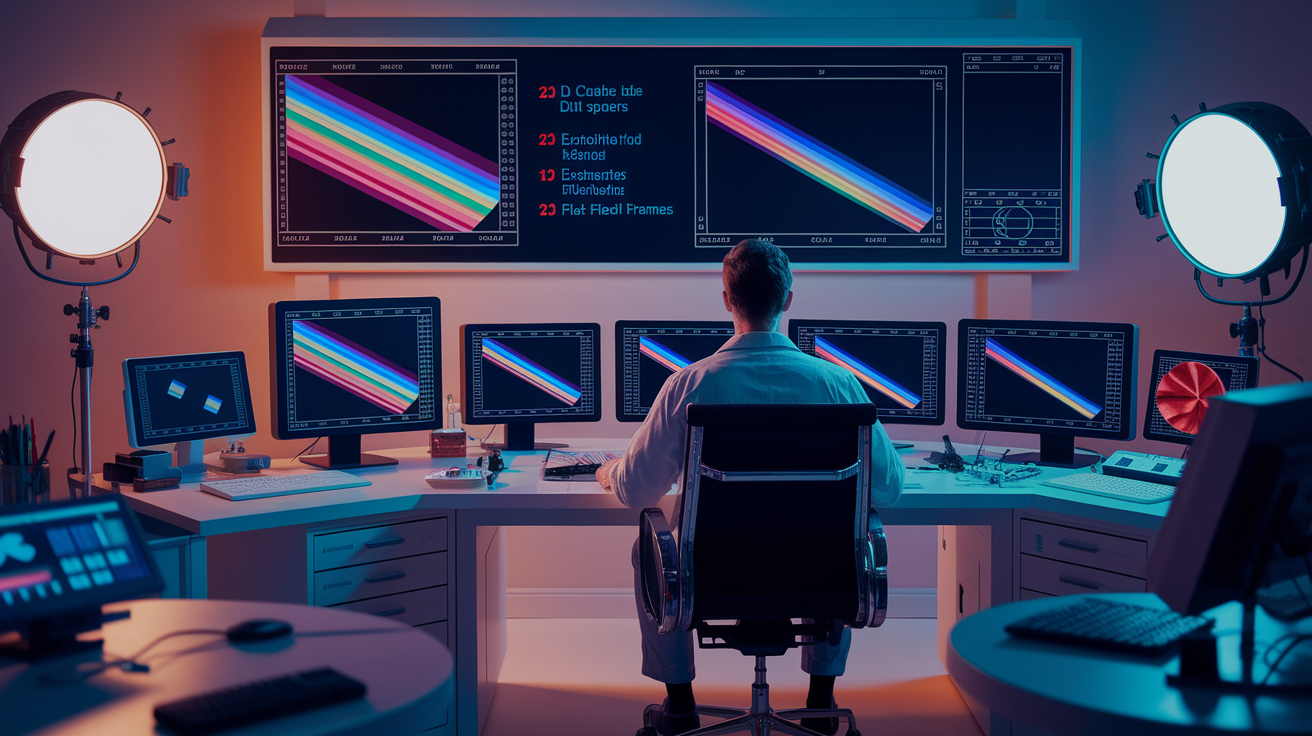
Workflow for Obtaining and Processing Stellar Spectra
Raw detector images hold more than starlight. Every pixel carries a small electronic offset, sensitivity varies across the chip, cosmic rays leave bright speckles. Processing fixes these before you can trust wavelength positions.
Standard reduction goes like this:
- Collect raw exposures. Point the telescope at your target, open the shutter for the planned time, save the CCD frame. Grab calibration lamp exposures and flat-field images through a uniform light source.
- Remove detector noise. Subtract the bias frame (zero-second exposure showing electronic offset) from each science and calibration frame to kill the baseline count.
- Correct pixel sensitivity. Divide by a normalized flat-field image to handle variations in pixel response plus any dust or vignetting.
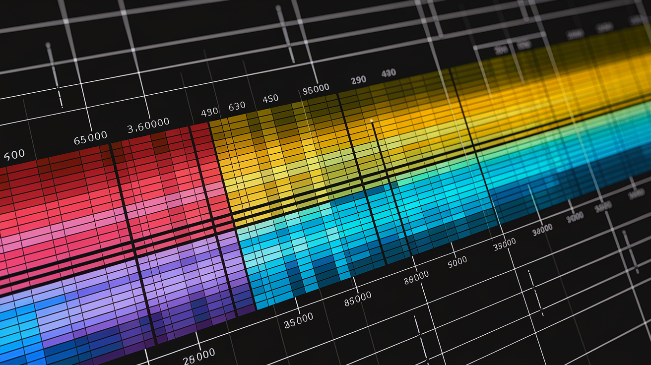
- Extract echelle orders. Trace the curved spectral orders on the two-dimensional frame, sum flux within each order, producing one-dimensional arrays of intensity versus pixel column.
- Apply wavelength calibration. Match pixel positions of known lamp lines to lab wavelengths, fit a polynomial or spline mapping pixel number to wavelength for every order.
- Produce a final normalized spectrum. Divide the extracted star spectrum by a smooth continuum model so absorption lines dip from a baseline near one, making depths and shifts easier to measure.
After that you’ve got a calibrated, one-dimensional spectrum ready for velocity extraction. Each wavelength bin has a known value in nanometers or angstroms, flux is a fraction of the continuum. Clean dataset ready for cross-correlation or line fitting.
Wavelength Calibration and Reference Standards

Absolute wavelength accuracy controls how well you convert a measured shift into velocity. Even a 0.01 nm error at 500 nm translates to 6 km/s. Not acceptable for exoplanet work. Calibration lamps and laser systems provide stable, known lines anchoring your wavelength solution.
Three reference types run modern practice. Thorium-argon hollow-cathode lamps spit out hundreds of emission lines across the optical band. Easy to run, give wavelength precision around 20 to 50 centimeters per second over short times, but lamp aging and pressure shifts drift things long term. Iodine absorption cells drop a forest of narrow molecular lines straight into the stellar beam. Because iodine lines mix with the star’s spectrum, any instrumental shift hits both equally, so you can track and remove drift. Precision reaches 1 to 2 meters per second, but iodine only works in the 500 to 620 nm window and makes reduction messier. Laser frequency combs create a regular grid of lines locked to an atomic clock. They cover broader ranges and hit stability below 1 centimeter per second, making them the reference for next-gen surveys chasing Earth-analog planets.
| Reference Type | Precision Level | Typical Use |
|---|---|---|
| Th–Ar lamp | 20–50 cm/s | General RV surveys, binary stars |
| Iodine cell | 1–2 m/s | Exoplanet detection (500–620 nm band) |
| Frequency comb | <1 cm/s | Ultra-stable campaigns, Earth-analog searches |
Measuring Line Shifts and Computing Velocity
Once your spectrum’s calibrated, you need to measure how far each line moved from its rest position. Two methods dominate. Line-by-line fitting treats each absorption feature solo: identify a line, fit a Gaussian or Voigt profile to its shape, record the centroid wavelength, compare to the lab value. Repeat for dozens or hundreds of lines, take a weighted average of the individual velocity measurements. Works well when lines are isolated and strong, lets you inspect each feature for blends or asymmetries that might skew things.
Cross-correlation treats the whole spectrum as one pattern. You compute the cross-correlation function between your observed spectrum and a high-quality template (synthetic model or a high-signal observation of the same star). The CCF peaks at the velocity shift that best lines up the two spectra. This leverages all lines at once, boosting precision when signal-to-noise is modest. Trade-off is that blended or wonky lines add noise to the CCF, and you have to pick or build a template matching the star’s spectral type and broadening. Lots of pipelines mix both, using cross-correlation for the bulk measurement and line fitting to check individual features or study line-shape changes.
Velocity accuracy hangs on spectral resolution and signal-to-noise. Higher resolution spreads a line over more pixels, so you can nail the centroid tighter. Higher SNR cuts scatter in each pixel’s flux, shrinking uncertainty on the fit. Converting the measured shift to velocity is straightforward: compute Δλ/λ, multiply by c, result is v in the same units as c. If c’s in kilometers per second, v comes out in kilometers per second. For a shift of 0.001 nm at 600 nm, Δλ/λ is about 1.7×10⁻⁶, so v is roughly 0.5 km/s or 500 m/s. Watch the sign. Blueshift means approaching, redshift means receding.
Sources of Error and Noise in Radial Velocity Measurements
Stellar jitter comes from the star itself. Convective cells rise and fall, producing velocity signals on timescales of minutes to hours with amplitudes around 1 meter per second for Sun-like stars. Acoustic oscillations (p-modes) add another meter per second of scatter over 5 to 15 minute windows. Magnetic activity (spots and plages rotating across the visible face) can fake or hide planetary signals at the several meter per second level, especially for young or active stars. These astrophysical noise sources set a floor no instrument upgrade can break. You handle them by averaging over longer exposures, modeling activity indicators, or using multi-wavelength observations that separate chromatic from achromatic shifts.
Instrumental drift happens when the spectrograph’s optical alignment shifts between or during exposures. Temperature swings, mechanical flexure, air-pressure changes all nudge the spectrum on the detector by fractions of a pixel. Without correction, drifts look like false velocity wiggles. Simultaneous calibration (recording a reference spectrum through the same optics at the same time as the star) tracks and kills most drift. Photon noise stems from the finite number of photons collected. Fewer photons mean bigger counting uncertainties, which spread into the wavelength centroid and velocity measurement. Doubling exposure time roughly halves photon noise, but only if stellar jitter and sky background don’t take over first.
Common error contributors:
- Stellar surface convection and granulation (0.3 to 1 m/s)
- Acoustic oscillations or p-modes (about 1 m/s, 5 to 15 min periods)
- Magnetic activity like spots, plages, cycles (several m/s, days to years)
- Instrumental temperature or pressure drifts (sub-meter per second to meters per second if uncorrected)
- Photon statistics, depends on target brightness, exposure time, detector efficiency
Applications of Radial Velocity Measurements
Radial velocity gave us the first confirmed exoplanet around a Sun-like star when observers caught a 50 meter per second periodic wobble in 51 Pegasi. Since then the method’s found over a thousand planets, especially massive ones in short orbits that make large, fast signals. Fitting the velocity curve to a Keplerian model pulls out the planet’s orbital period, the semi-amplitude of the star’s motion, and orbital eccentricity. Semi-amplitude K plus the star’s mass gives you the planet’s minimum mass (specifically M times sin of the orbital inclination). If the orbit’s edge-on, you get true mass. If it tilts toward face-on, the measured value underestimates reality. Combine radial velocity with transit photometry and you break this degeneracy, getting true mass, radius, bulk density.
Binary star systems throw much bigger velocity swings, often kilometers per second, making them easier to spot and nail down. Measuring radial velocities of both components over a full orbit lets you compute the mass ratio and, if you know the distance and catch eclipses, individual masses to a few percent. Spectroscopic binaries with periods of days to years fill stellar-mass catalogs and test evolution models. On bigger scales, radial velocities of stars in a galaxy trace its rotation curve and velocity dispersion. Observations showing rotation speeds stay high far from galactic centers gave early dark matter evidence. Precision for these runs from sub-meter per second for exoplanet surveys to hundreds of kilometers per second for distant galaxies. But the core technique stays put: measure the Doppler shift, apply the formula, read the velocity.
Final Words
We traced how a star’s motion shows up as tiny wavelength shifts, and why precision instruments and careful calibration are needed to measure them.
You saw the workflow, collecting spectra, cleaning them, calibrating with lamps or combs, then fitting lines or using cross-correlation to get velocity. We also flagged main error sources, like stellar jitter, instrument drift, and photon noise, so you know the limits.
Putting it together, this guide shows how to measure stellar radial velocity using Doppler spectroscopy step by step, from telescope to final km/s value. Try it on a simple target first. With patience and care you can get useful results.
FAQ
Q: What is radial velocity measurements using Doppler spectroscopy?
A: The radial velocity measurement using Doppler spectroscopy is the line-of-sight speed of a star or object, given in km/s, found from spectral line shifts: blueshift means approach, redshift means recession.
Q: How do you calculate velocity using the Doppler effect and how do you measure radial velocity?
A: You calculate velocity using the Doppler effect by measuring the fractional wavelength shift Δλ/λ = v/c and solving for v; practically you compare observed and rest wavelengths after careful calibration and cross-correlation.