
What if you could tell how fast a star or galaxy is moving just by measuring tiny shifts in its light?
That’s the Doppler shift (a change in wavelength caused by motion), the same idea behind a passing siren, and it turns spectral fingerprints, sharp lines from atoms, into simple speedometers.
This post shows, step by step, how to measure those wavelength shifts in spectra, convert them into redshift or blueshift and then into radial velocity, plus when the simple v ≈ c × z formula is fine and when you need the relativistic correction.
Core Principles Behind Doppler Shift Applied to Spectral Velocity Measurements

When a fire truck races toward you with its siren blaring, the pitch sounds higher. It drops as the truck speeds away. That shift happens because motion compresses or stretches the sound waves reaching your ears.
Light does the same thing. When a star, galaxy, or any glowing object moves toward Earth, its light gets squeezed to shorter wavelengths. That’s blueshift. When it moves away, wavelengths stretch longer. That’s redshift. This wavelength shift is the Doppler effect, and it gives astronomers a direct way to clock how fast distant objects are moving along our line of sight.
In a spectrum, every chemical element leaves a distinct pattern. Dark absorption lines or bright emission lines appear at precise rest wavelengths. When the source moves, those lines shift. The displacement Δλ = λobs − λrest is what you measure. Hydrogen’s alpha line sits at a rest wavelength of 656.3 nm in a stationary lab. If you observe that line at 660.0 nm in a star’s spectrum, the star is receding. The ratio of that shift to the rest wavelength defines the redshift z = Δλ / λrest. For speeds much slower than light, radial velocity is simply v ≈ c × z, where c is the speed of light, roughly 300,000 km/s. Plug in the hydrogen example: z = (660.0 − 656.3) / 656.3 ≈ 0.00564, so v ≈ 300,000 × 0.00564 ≈ 1,692 km/s. Round it to 1,800 km/s.
To extract a velocity from a spectrum, you need five quantities:
- Rest wavelength (λrest): the laboratory wavelength when the source is at rest.
- Observed wavelength (λobs): the wavelength you read from the spectrum after the Doppler shift.
- Wavelength shift (Δλ): the difference λobs − λrest, positive for redshift, negative for blueshift.
- Redshift (z): the dimensionless ratio Δλ / λrest that scales the velocity.
- Radial velocity (v): the speed along the line of sight, computed as c × z for non‑relativistic motion.
Practical Spectral Line Measurement for Doppler Velocity Extraction

Spectra can be displayed as a colored ribbon or as a line plot with intensity on the vertical axis and wavelength on the horizontal. Line plots are far more useful for velocity work. They let you read exact intensities, spot faint lines, and measure the peak or centroid of each feature precisely. A ribbon might look nice, but hovering over it to read a wavelength is guesswork. Weak lines disappear into the background. Modern detectors record intensity at thousands of wavelength points, and software converts those digital counts directly into line plots. An A-type star spectrum covering 3,500 to 4,200 Å reveals strong hydrogen absorption lines. You can zoom in on any feature and measure its position to a fraction of an angstrom.
The measurement procedure is straightforward. First, identify a known spectral line. Hydrogen beta at 4,860 Å is common in galaxy spectra. The hydrogen alpha line at 656.3 nm works well for stars. Next, locate that line in the observed spectrum and read the wavelength λobs of its absorption or emission peak. Compute the shift Δλ = λobs − λrest. From that shift, calculate the redshift z = Δλ / λrest and then the velocity v = c × z. The sign of Δλ tells you the direction: positive means the object is receding, negative means it’s approaching.
| Quantity | Description |
|---|---|
| λrest | Laboratory rest wavelength of the spectral line (Å or nm) |
| λobs | Observed wavelength measured from the spectrum (Å or nm) |
| Δλ | Wavelength shift = λobs − λrest (positive for redshift, negative for blueshift) |
| z | Dimensionless redshift = Δλ / λrest |
Using Doppler Formulas: Non‑Relativistic and Relativistic Velocity Relations
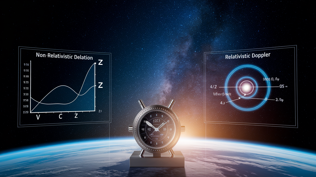
When an object’s velocity is much smaller than the speed of light, say a few thousand kilometers per second or less, the simple formula v ≈ c × z works fine. Here z = Δλ / λrest, and you can take c as 3.0 × 10⁵ km/s for convenience or 3.0 × 10⁸ m/s if you prefer metric. This approximation breaks down when speeds climb above a few percent of c. Special relativity warps the relationship between wavelength shift and velocity.
For high velocities, you must use the full relativistic Doppler formula: λobs / λemit = sqrt((1 + v/c) / (1 − v/c)). You can rearrange this to solve for v in terms of the measured wavelength ratio. The relativistic correction matters for distant galaxies with large redshifts and for any object moving at a significant fraction of light speed. Below a few thousand km/s, the non‑relativistic approximation introduces negligible error and keeps calculations simple.
Worked Velocity Examples Using Doppler Shift in Real Astronomical Spectra
To measure a velocity, start by isolating a clean spectral line with a known rest wavelength. Read the observed wavelength from your spectrum. Subtract the rest wavelength to get the shift Δλ. Divide that shift by the rest wavelength to find z. Multiply z by the speed of light to get the radial velocity.
Take Galaxy A. You observe the hydrogen beta emission line and measure its wavelength at 4,950 Å. The rest wavelength of hydrogen beta is 4,860 Å. The shift is Δλ = 4,950 − 4,860 = 90 Å. The redshift is z = 90 / 4,860 ≈ 0.0185. Multiply by c = 3.0 × 10⁵ km/s and you get v = 0.0185 × 300,000 = 5,550 km/s. The positive velocity means Galaxy A is receding from us at about 5,550 km/s. That’s a typical recessional speed for a distant galaxy in an expanding universe.
Now consider a stellar example. A star’s hydrogen alpha line has a rest wavelength of 656.3 nm. You measure it at 660.0 nm in the star’s spectrum. The shift is Δλ = 660.0 − 656.3 = 3.7 nm. The redshift is z = 3.7 / 656.3 ≈ 0.00564, so v ≈ 0.00564 × 300,000 ≈ 1,692 km/s. Round it to 1,800 km/s. Before precision spectrographs existed, astronomers could miss a star’s motion entirely if its velocity was only a few kilometers per second. Today, shifts smaller than a meter per second are routinely detected. The sign tells you the star is moving away. The magnitude tells you how fast. A velocity of several hundred to a few thousand km/s is common for stars in the Milky Way or for galaxies at moderate distances.
To apply this method, follow these steps:
- Identify the spectral line and look up its laboratory rest wavelength.
- Measure the observed wavelength from the spectrum’s peak or centroid.
- Compute the wavelength shift Δλ and the redshift z.
- Calculate the radial velocity v = c × z and note the sign to determine direction.
Doppler Velocities in Stellar and Binary‑Star Systems
Stars in binary systems orbit a common center of mass. That orbital motion produces periodic Doppler shifts in their spectral lines. When one star swings toward Earth, its lines shift blueward. When it swings away, they shift redward. If you measure the star’s spectrum over weeks or months, the wavelength of any given line oscillates with the orbital period. The amplitude of that oscillation depends on the star’s orbital speed and the inclination of the orbit. Edge‑on systems show the maximum Doppler effect. Face‑on orbits produce almost no measurable shift because the motion is perpendicular to our line of sight. By tracking these radial‑velocity curves, astronomers can determine orbital periods, component masses, and even detect unseen companions that tug on the visible star.
Stellar rotation also leaves a Doppler signature, but instead of shifting lines, it broadens them. The side of a rotating star that spins toward us emits slightly blueshifted light. The side spinning away emits redshifted light. When you observe the whole disk at once, the spectral line is smeared across a range of wavelengths. The width of that smear depends on the star’s rotation speed and the angle at which you view the rotation axis. If the axis points nearly toward you, the measured broadening is small even if the star spins rapidly. Other processes can also broaden lines. Turbulence, stellar winds, and magnetic fields all contribute, so careful analysis is needed to isolate the rotational component.
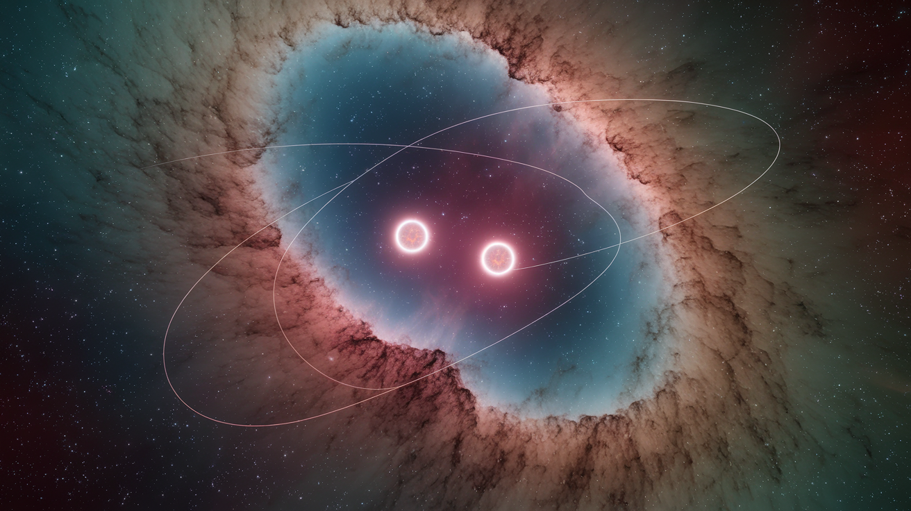
Line Splitting in Spectroscopic Binaries
When two stars of similar brightness orbit edge‑on, their spectral lines can split into distinct pairs. As one star approaches and the other recedes, the approaching star’s absorption line shifts blue and the receding star’s shifts red. If the stars are bright enough and the velocity separation large enough, you see two separate lines oscillating back and forth in wavelength. At maximum separation, when one star is directly approaching and the other directly receding, the lines are farthest apart. When both stars cross perpendicular to the line of sight, the lines merge. This line‑doubling technique was the first method to reveal that many apparently single stars are actually close binary systems.
Detecting Exoplanets with Doppler Spectroscopy
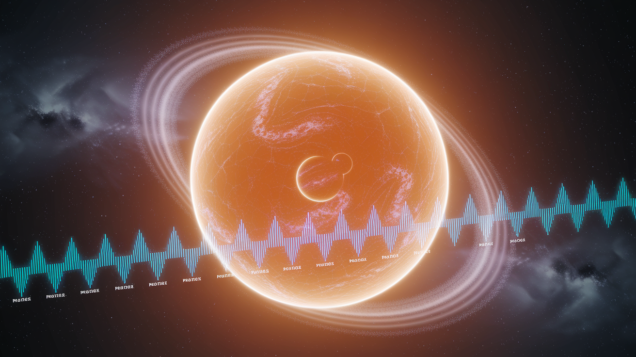
A planet orbiting a star doesn’t just sit still. It tugs the star into a small orbit around the system’s center of mass. That wobble shifts the star’s spectral lines by tiny amounts. When the planet pulls the star toward us, the lines shift blue. When it pulls the star away, the lines shift red. The first exoplanet detected around a Sun‑like star, 51 Pegasi b, was discovered in 1995 by measuring these periodic radial‑velocity shifts. The amplitude of the wobble is proportional to the planet’s mass and inversely related to its orbital distance. A massive planet close to its star, a “hot Jupiter,” can induce velocity shifts of tens or hundreds of meters per second. That’s easily detectable with modern spectrographs. Earth‑like planets in habitable zones produce wobbles smaller than 1 meter per second, which pushes the limits of current precision.
The periodic pattern of the velocity signal reveals the planet’s orbital period directly. Fit a sine wave to the radial‑velocity data. The period tells you how long the planet takes to orbit. The amplitude, combined with the star’s mass, gives the minimum mass of the planet. Minimum, because you only measure the component of the orbit projected along your line of sight. If the orbit is tilted face‑on, the true mass is larger. Over time, repeated observations build up a radial‑velocity curve that can reveal multiple planets, eccentric orbits, and even hints of moons or rings.
Three main challenges complicate Doppler exoplanet detection:
- Stellar activity: Star spots, flares, and convection cells create noise in the spectral lines that can mimic or mask planetary signals, especially for low‑mass planets.
- Inclination ambiguity: Without additional data, such as a transit, you can’t measure the orbital tilt. The derived planet mass is always a lower limit.
- Precision requirements: Detecting Earth‑mass planets requires velocity measurements stable to better than 1 m/s over years. That demands exquisite wavelength calibration and long‑term instrument stability.
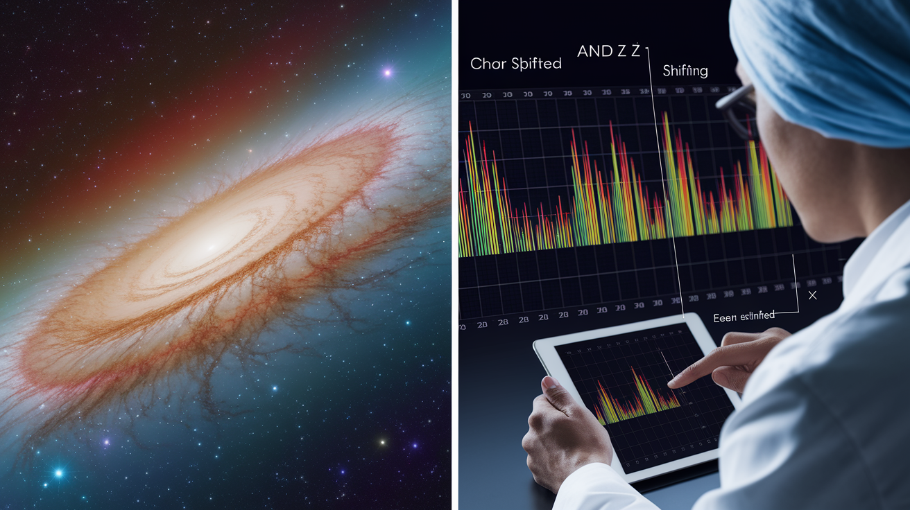
Galaxy Rotation, Cosmological Redshift, and Dark Matter Connections

When you point a spectrograph at different parts of a spiral galaxy and measure Doppler shifts, you map out how the galaxy rotates. One side of the disk approaches, shifting its spectral lines blue. The other side recedes, shifting them red. Plot the measured velocity against the distance from the galaxy’s center and you get a rotation curve. For a simple gravitating mass concentrated at the center, you’d expect the velocity to drop off with radius, just like planets orbiting the Sun. But real galaxies show rotation curves that stay flat or even rise far beyond the visible disk. That flat profile means there’s additional unseen mass spread throughout and beyond the luminous stars. We call that extra mass Dark Matter. Doppler mapping of galaxy rotation provided some of the earliest strong evidence for its existence. Current estimates put Dark Matter at roughly 26.5% of the total mass‑energy of the Universe.
Cosmological redshift is a related but distinct phenomenon. When light travels across billions of light‑years of expanding space, the wavelengths are stretched not by the source’s motion through space, but by the expansion of space itself. For nearby galaxies moving at a few thousand km/s, the distinction hardly matters. Both effects produce a redshift. But at large distances and high redshifts, cosmological expansion dominates, and you must interpret z in terms of scale‑factor growth rather than simple velocity. Gravitational redshift is yet another effect: photons climbing out of a deep gravitational potential lose energy and shift to longer wavelengths. All three processes change observed wavelengths, but their physical origins are different.
| Effect | Physical Origin | Typical Context |
|---|---|---|
| Doppler shift | Motion of source relative to observer | Stars, binaries, nearby galaxies, rotation curves |
| Cosmological redshift | Expansion of space stretching wavelengths | Distant galaxies, large‑scale structure, Hubble flow |
| Gravitational redshift | Photon energy loss in strong gravitational fields | White dwarfs, neutron stars, near black holes |
Corrections, Calibration, and Uncertainty in Doppler Velocity Measurements

Raw wavelength measurements from a spectrograph are never perfect. The instrument itself has a zero‑point offset, a small systematic shift caused by optical alignment, detector response, or temperature drift. You remove this offset by observing calibration lamps with known emission lines before, after, or simultaneously with your science target. Telluric lines, absorption features from Earth’s atmosphere, contaminate the spectrum and must be identified and masked or modeled out. And Earth is moving. It orbits the Sun, and the Sun orbits the galaxy. If you measure a star’s velocity without correcting for Earth’s motion, you’re mixing the star’s true velocity with our own. The barycentric correction shifts your measured velocity into the frame of the solar system’s center of mass. The heliocentric correction shifts it to the Sun’s frame. Both corrections can reach tens of kilometers per second and must be applied before you can compare velocities measured on different nights.
Uncertainties in Doppler velocities come from several sources. Photon noise limits how precisely you can measure a line’s centroid. Faint spectra have noisier peaks. Calibration drift introduces systematic errors if your wavelength solution changes between the calibration exposure and the science exposure. Blended lines, broad features, and asymmetric line profiles make centroid measurements ambiguous. Stellar activity, pulsations, and granulation add real scatter. To estimate your velocity uncertainty, propagate the wavelength measurement error through the Doppler formula, combine it with calibration uncertainties, and check for scatter in repeated observations of the same target. Cross‑correlation techniques and template matching can improve precision by using many lines at once rather than relying on a single feature.
The main uncertainty sources in radial‑velocity work are:
- Photon noise: limited signal‑to‑noise ratio in the spectrum makes line positions harder to measure.
- Wavelength calibration drift: changes in the spectrograph between calibration and science exposures introduce systematic shifts.
- Line blending and asymmetry: overlapping lines or intrinsic profile shapes bias centroid measurements.
- Telluric contamination: atmospheric absorption lines can shift or distort stellar features if not properly removed.
- Stellar variability: intrinsic changes in the star’s spectrum, spots, pulsations, convection, add scatter to the measured velocities.
Final Words
We walked through how motion changes spectral lines—starting with a sound analogy, spotting redshift versus blueshift, and measuring λrest and λobs to get Δλ.
You saw the key formulas (Δλ = λobs − λrest; v ≈ c·Δλ/λrest or the relativistic form), step-by-step examples, and why calibration and corrections matter for accuracy.
With those ingredients, Doppler shift and measuring velocity from spectra becomes a practical way to map motion in stars, planets, and galaxies. Keep practicing—the method pays off.
FAQ
Q: What is Doppler shift and how does motion change observed wavelength?
A: The Doppler shift is the change in observed wavelength caused by relative motion between source and observer, like pitch change for sound; motion toward shortens wavelengths (blueshift), away lengthens them (redshift).
Q: How is Doppler shift converted into velocity?
A: The Doppler shift converts to velocity using v ≈ c × (Δλ/λrest), where Δλ = λobs − λrest and c ≈ 300,000 km/s; this non‑relativistic formula holds when v is much less than c.
Q: When should I use the relativistic Doppler formula?
A: You use the relativistic Doppler formula when speeds approach a significant fraction of light speed; then λobs/λemit = sqrt((1+v/c)/(1−v/c)), solved numerically for v.
Q: What measurements are required to determine radial velocity from a spectrum?
A: To measure radial velocity you need the rest wavelength, observed wavelength, Δλ, redshift z, and the velocity v derived from Δλ or z using the Doppler relation.
Q: How do you measure the observed wavelength (λobs) in a spectrum?
A: Measuring λobs requires a line plot spectrum: identify a known element’s fingerprint line, read the peak wavelength from the plot, and record λobs for Δλ calculation.
Q: Can you give a worked hydrogen alpha example?
A: Using the hydrogen alpha example, the rest λ is 656.3 nm and observed λ 660.0 nm; Δλ = 3.7 nm gives v ≈ 1,800 km/s using v ≈ c(Δλ/λrest).
Q: How does Doppler spectroscopy detect exoplanets?
A: Exoplanets are detected by periodic Doppler shifts: planets tug stars, producing tiny, repeating radial‑velocity changes that reveal orbital period and a minimum planet mass from amplitude.
Q: What corrections and uncertainties affect Doppler velocity measurements?
A: Corrections and uncertainties include instrument zero‑point, barycentric (Earth motion) correction, telluric line removal, photon noise, and calibration drift—each affects the final velocity precision.
Q: How do Doppler velocities reveal galaxy rotation and dark matter?
A: Doppler mapping measures galaxy rotation by sampling velocities across a disk; flat rotation curves indicate extra unseen mass, which points to dark matter presence and distribution.
Q: What is the difference between cosmological redshift and Doppler motion?
A: Cosmological redshift differs from Doppler motion: cosmological redshift stretches wavelengths through space expansion, while Doppler shifts come from local relative motion of source and observer.
Q: How do Doppler methods show motion in binary stars?
A: Spectroscopic binaries show alternating line shifts or splitting as stars orbit; edge‑on systems produce largest radial‑velocity swings, while rotation broadens lines and inclination reduces measured speed.