
Think spectral lines are perfectly sharp fingerprints of atoms? Not true.
Real stars smear those lines, and that smear carries real physics.
This post explains what causes spectral line broadening in stars—focusing on temperature, pressure, and rotation.
Temperature means thermal Doppler motion (atoms moving fast and shifting light).
Pressure means frequent collisions that shorten excited-state lifetimes.
Rotation means different parts of the visible disk shift light toward or away from us.
I’ll show how each effect changes line shape and what that tells us about a star’s temperature, density, and spin.
Core Physical Causes Behind Stellar Spectral Line Broadening
Spectral line broadening is what happens when absorption or emission features in stellar spectra spread out beyond the infinitesimally narrow wavelengths you’d expect from simple atomic physics. No real star shows perfectly sharp spikes. Every line gets smeared across some measurable wavelength range, and that smearing tells you about the physical conditions in the stellar atmosphere. Temperature, pressure, motion, turbulence—they all leave their marks in how wide a line becomes and what shape it takes.
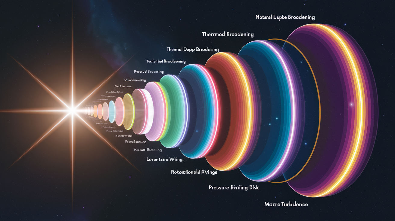
Five big things drive what causes spectral line broadening in stars: quantum-mechanical limits on atomic transitions, thermal motion of atoms, collisions between particles in dense gas, bulk rotation of the stellar surface, and turbulent velocity fields inside the atmosphere. Natural (quantum) broadening sets a baseline minimum width, determined by the Heisenberg uncertainty principle and how long excited atomic states stick around. Thermal Doppler broadening comes from atoms zipping around at random velocities tied to temperature, creating a spread that maps directly to kinetic energy. Pressure (collisional) broadening kicks in where atoms and ions bump into each other constantly, messing with energy levels and cutting short state lifetimes. Rotational broadening from stellar spin creates different Doppler shifts across the visible disk, stretching lines asymmetrically. Macroturbulence in stellar atmospheres throws in large-scale convective or wave-driven velocity fields that widen profiles even further.
Observers usually sort broadened lines by their math shapes. Gaussian profiles typically point to velocity-driven broadening (thermal or turbulent), Lorentzian wings mean collision- or lifetime-dominated broadening, and Voigt profiles are a mix of both. Each mechanism works in parallel. The observed line shape is the sum of everything that’s active.
Five primary broadening mechanisms:
- Natural broadening: Intrinsic quantum width from finite excited-state lifetimes. Usually the smallest contribution.
- Thermal Doppler broadening: Velocity spread from temperature. Produces Gaussian profiles with widths of a few to tens of km/s.
- Pressure (collisional) broadening: Interaction-driven widening that dominates in high-density layers. Creates extended Lorentzian wings.
- Rotational broadening: Doppler shifts across a spinning stellar disk. Can hit hundreds of km/s in rapid rotators.
- Macroturbulence: Large-scale atmospheric motions. Adds velocity-equivalent widths of a few to tens of km/s.
Thermal Doppler Broadening in Stellar Atmospheres
Thermal Doppler broadening happens because atoms in a stellar atmosphere don’t sit still. They move in random directions with velocities set by temperature. An atom moving toward you emits or absorbs light that’s slightly blueshifted. One moving away produces a redshift. When billions of atoms contribute, their individual Doppler shifts blend into a single broadened line profile. The velocity distribution follows Maxwell–Boltzmann statistics, so the resulting line shape is Gaussian. The width of this Gaussian (measured as full width at half maximum in velocity units) scales as the square root of temperature divided by atomic mass. Hotter gas or lighter atoms mean wider lines.
Thermal Doppler broadening dominates the intrinsic width of many stellar lines, especially in hot stars with low atmospheric densities. For hydrogen in a 10,000 K photosphere, thermal velocities correspond to Doppler widths near 20 km/s. At 10,000 K, hydrogen atoms race at thermal speeds that broaden spectral lines by roughly 20 km/s, enough to smear a sharp fingerprint into a measurable blur. Heavier elements like iron show narrower thermal widths at the same temperature because their greater mass reduces typical velocity. Measuring the Doppler width of a line from a known element lets astronomers estimate the temperature of the emitting or absorbing layer, making thermal broadening a key diagnostic tool.
Temperature regime examples:
- Cool stars (3,000–4,000 K): Thermal Doppler widths for heavy elements run around 2–4 km/s. Molecular lines also present with similar or slightly larger widths.
- Solar-type stars (~5,800 K): Iron and other metals show thermal widths around 3–6 km/s. Hydrogen lines reach about 10 km/s.
- A/B stars (10,000–20,000 K): Thermal widths for hydrogen climb to 20–30 km/s. Helium and heavier ions also broaden significantly.
- Very hot stars (>30,000 K): Hydrogen and ionized helium lines can exceed 40 km/s purely from thermal motion. Often blended with other effects.
Pressure and Collisional Broadening in Dense Stellar Layers
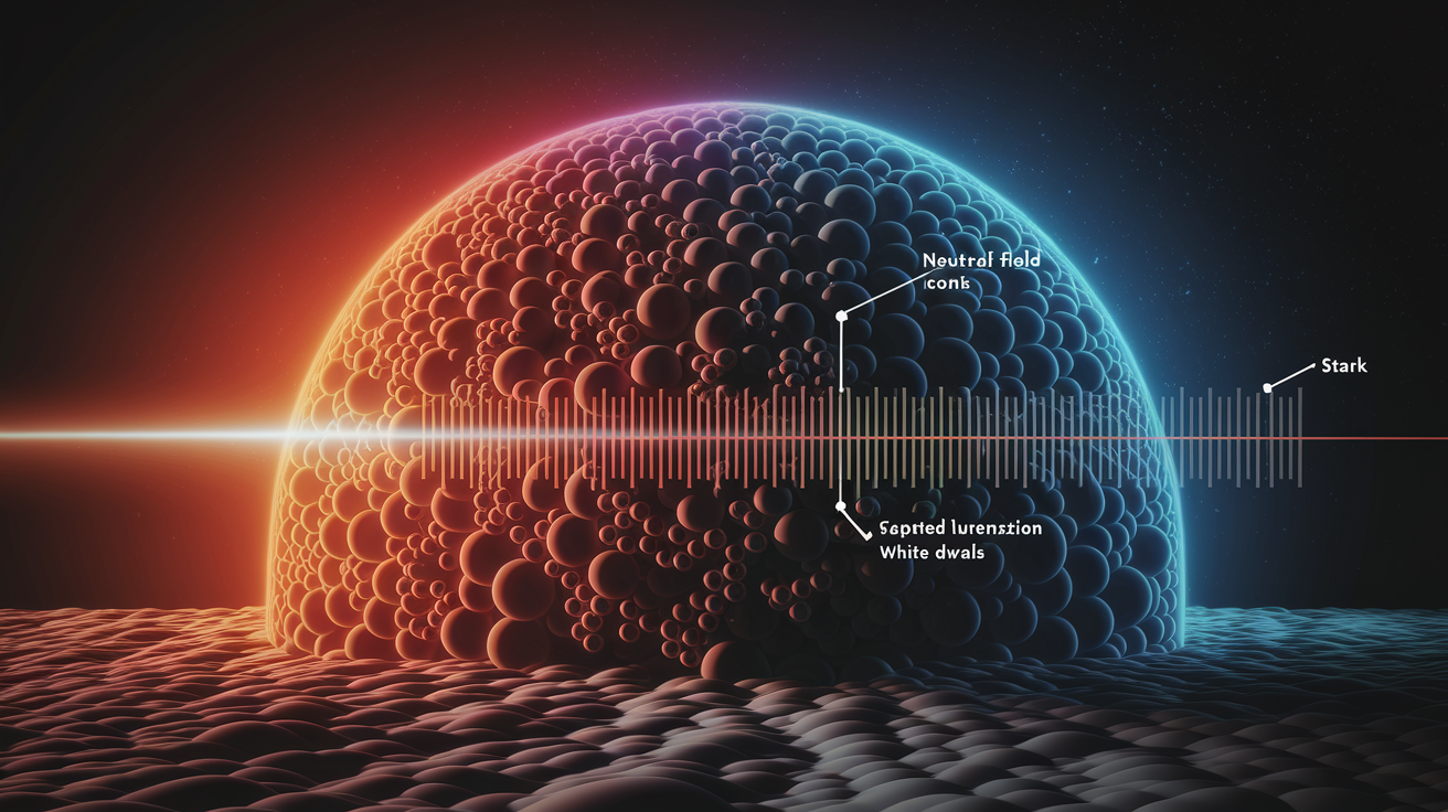
Pressure broadening occurs when atoms or ions collide or interact electromagnetically during the time they emit or absorb photons. These interactions mess with atomic energy levels and shorten the effective lifetime of excited states, both of which increase line width. Unlike thermal broadening, which produces a smooth Gaussian, collisional broadening generates Lorentzian wings (extended tails that fall off slowly with distance from line center). The strength of pressure broadening depends on the density of perturbing particles. Higher pressure means more frequent collisions and wider lines.
Two main types of collisional broadening dominate in different stellar environments. Stark broadening results from electric fields of nearby charged particles (electrons and ions) and is especially strong in hot, ionized atmospheres where free electrons are abundant. Van der Waals broadening arises from neutral-atom interactions and dominates in cooler stars where hydrogen remains mostly neutral. The hydrogen Balmer lines in A-type stars (around 10,000 K) show pronounced Stark wings shaped by high electron densities in the photosphere. Metal lines in cool K and M dwarfs exhibit van der Waals broadening from collisions with neutral hydrogen atoms.
White dwarfs represent an extreme case. Their surface gravities compress atmospheres to such high densities that pressure broadening overwhelms all other mechanisms. Hydrogen lines in white dwarfs can span tens or even hundreds of angstroms, with wings extending far from the line core. In white dwarf atmospheres, gravity squeezes gas so tightly that a single hydrogen line spreads across wavelengths wide enough to swallow dozens of normal stellar features. Measuring these enormous widths allows observers to estimate surface gravity and, by extension, stellar mass.
| Broadening Type | Dominant Environment |
|---|---|
| Stark (electron impact) | Hot stars, ionized plasmas, white dwarfs |
| Van der Waals (neutral collisions) | Cool main-sequence stars, giant atmospheres |
| Resonance broadening | Lines where lower level is ground state; density-sensitive |
Rotational Broadening From Stellar Spin
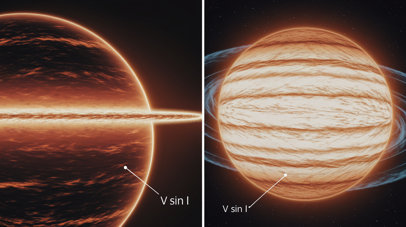
Rotational broadening from stellar spin creates line widening through a geometric Doppler effect. One limb of a rotating star moves toward the observer while the opposite limb recedes. Light from the approaching side blueshifts, light from the receding side redshifts. When integrated across the visible disk, these shifts blend into a single broadened profile. The amount of broadening depends on the projected equatorial velocity v sin i, where v is the true equatorial speed and i is the inclination angle between the rotation axis and the line of sight. A pole-on star (i = 0°) shows no rotational broadening. An equator-on star (i = 90°) reveals the full effect.
Slow rotators like the Sun produce modest rotational broadening (roughly 2 km/s at the solar equator), often buried beneath thermal Doppler and macroturbulent contributions. Rapidly rotating stars, common among young A- and B-type objects, can spin at hundreds of kilometers per second, producing dramatically widened and distinctively flattened line profiles. Limb darkening (the fact that a star’s edge appears dimmer than its center) modifies the profile shape slightly, causing the classic rotational profile to dip in the middle rather than staying perfectly flat.
Rotational velocity examples:
- Slow rotators (Sun-like stars): v sin i runs around 2–5 km/s. Rotational broadening usually smaller than thermal or macroturbulent widths.
- Moderate rotators (young solar analogs, some F stars): v sin i sits around 10–50 km/s. Rotation becomes a measurable component of total line width.
- Rapid rotators (A-type main sequence, Be stars): v sin i can exceed 200 km/s, creating very broad, shallow lines and enabling precise rotation-rate measurements.
Measuring rotational broadening serves multiple purposes. It constrains stellar age (rotation slows over time due to magnetic braking), tests models of angular-momentum evolution, and helps disentangle rotation from other broadening sources in spectral synthesis. When combined with period measurements from photometric variability, v sin i can yield stellar radius estimates and constrain the inclination angle i.
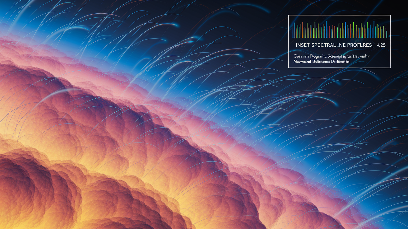
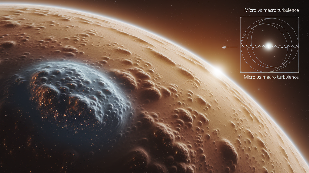
Turbulence and Velocity Fields: Micro- and Macroturbulent Broadening
Turbulent velocity fields in stellar atmospheres add another layer of line broadening beyond simple thermal motion and rotation. Microturbulence refers to small-scale, unresolved motions (typically on scales smaller than a photon’s mean free path) that increase the effective velocity spread of absorbing atoms. Because microturbulent velocities are random and isotropic, they broaden lines in a manner similar to thermal Doppler broadening, producing a Gaussian contribution. But microturbulence doesn’t depend on atomic mass, so it affects all spectral lines equally in velocity space, unlike thermal broadening which scales with √(T/M). Measuring how line width changes across elements of different masses allows observers to separate thermal and microturbulent components. Typical microturbulent velocities in solar-type stars range from 1 to 3 km/s.
Macroturbulence describes large-scale velocity fields (convective cells, granulation, or wave motions) on scales large enough that different parts of the stellar disk exhibit coherent velocity shifts. These bulk flows shift line centroids locally, and when integrated across the visible surface, they broaden the observed profile. Macroturbulence produces a velocity-equivalent width of a few to tens of km/s in many main-sequence and giant stars. Unlike rotation, which creates a characteristic flat-bottomed or smoothly sloped profile, macroturbulence tends to preserve a more rounded, Gaussian-like shape because the velocity field is more isotropic.
Disentangling macroturbulence from rotation requires careful profile analysis. One key diagnostic is the line bisector, a curve that traces the midpoint of the line profile at each depth. Rotational broadening typically produces symmetric bisectors, while macroturbulent and convective velocity fields can introduce asymmetries or C-shaped bisectors. Convective blueshift, a subtle wavelength shift caused by the correlation between bright, rising gas (blueshifted) and dark, sinking gas (redshifted) with different surface coverage, also appears in high-resolution spectra of stars with vigorous convection.
Diagnosing Turbulence in Line Shapes
Line bisectors and asymmetries serve as powerful tools to probe velocity structure in stellar atmospheres. A bisector is constructed by measuring the wavelength at half-maximum intensity on both sides of a line and plotting the midpoint as a function of line depth. In a star dominated by rotation alone, the bisector remains vertical or slopes gently. In a convective atmosphere, the bisector often curves, reflecting how rising (blueshifted) granules contribute more flux than sinking (redshifted) lanes. The curved bisector of a spectral line acts like a velocity map, revealing where hot gas rises and cool gas sinks across a star’s roiling surface. Convective blueshift is measured as a small but systematic offset of line cores toward shorter wavelengths, typically a few hundred meters per second in the Sun and up to a few km/s in more active stars. These diagnostics, combined with radiative-transfer models that simulate granulation and convection, allow astronomers to measure macroturbulent velocities and test hydrodynamic predictions of stellar atmospheres.
Magnetic, Quantum, and Additional Broadening Mechanisms in Stars
Natural (quantum) broadening sets the fundamental lower limit on spectral line width, arising from the Heisenberg uncertainty principle: ΔE Δt ≥ ħ/2. Because excited atomic states have finite lifetimes Δt, their energies are uncertain by ΔE, which translates into a minimum wavelength spread. For most optical transitions, natural widths are extremely small (on the order of 10⁻⁴ Å or less), far narrower than thermal, pressure, or rotational contributions. Natural broadening becomes significant only in special cases, such as very strong resonance lines or environments where all other broadening mechanisms are suppressed. Natural broadening is almost always negligible in stellar spectra and serves mainly as a theoretical baseline.
Zeeman splitting introduces a different kind of line modification in the presence of magnetic fields. A magnetic field splits degenerate atomic energy levels into multiple sublevels, each corresponding to a slightly different photon energy. The result is that a single spectral line divides into two or more closely spaced components. If the magnetic field is strong and the spectral resolution high, individual Zeeman components appear as separate lines. If the field is weaker or resolution lower, the components blend into an apparently broadened or polarized profile. Measuring Zeeman broadening and polarization allows observers to map magnetic field strengths and geometries on stellar surfaces, a technique widely used in studies of magnetic A and B stars, cool-star spots, and the Sun.
Hydrogen Balmer lines (especially Hα, Hβ, and Hγ) show particularly strong broadening in hot stars because they combine large intrinsic oscillator strengths with sensitivity to both Stark and thermal effects. In A-type stars near 10,000 K, Balmer lines dominate the optical spectrum and serve as primary temperature and gravity diagnostics. Their broad, pressure-sensitive wings encode information about photospheric electron density. Molecular line broadening becomes important in cool stars (M dwarfs, giants, and supergiants) where molecules like TiO, H₂O, and CO form. Molecular bands consist of many closely spaced rotational and vibrational lines. Their effective broadening reflects both the intrinsic structure of the band and the same physical mechanisms (thermal, pressure, turbulence) that affect atomic lines. Line blending in crowded spectra adds another layer of complexity. When two or more lines lie close in wavelength, their profiles overlap, creating an apparently broader or distorted feature that must be deconvolved during analysis.
Additional broadening contributors:
- Zeeman splitting: Magnetic fields divide lines into polarized components. Field strengths of a few hundred gauss to several kilogauss produce measurable splitting or broadening.
- Natural broadening: Quantum-limited width from finite state lifetimes. Negligible in most stellar contexts but sets a fundamental floor.
- Molecular bands: Overlapping rotational-vibrational lines in cool stars. Effective broadening can reach tens of km/s equivalent width.
- Line blending: Unresolved line overlap in metal-rich or cool stars. Requires careful modeling to separate individual contributions.
Instrumental Effects and Observational Broadening in Spectroscopy
Instrumental profile effects introduce artificial broadening that must be carefully separated from astrophysical signals. Every spectrograph has a finite spectral resolution, characterized by the resolving power R = λ/Δλ, where Δλ is the smallest wavelength difference the instrument can distinguish. A spectrograph with R = 50,000 at 5000 Å resolves features separated by 0.1 Å, corresponding to a velocity resolution of about 6 km/s. Any astrophysical line narrower than this limit will appear broadened to the instrument’s resolution. The instrumental line spread function describes how a delta-function input line (an infinitely narrow spike) spreads into the observed profile. This function is typically Gaussian or nearly Gaussian, determined by slit width, grating or prism dispersion, detector pixel size, and optical aberrations.
High-resolution spectroscopy, with R above about 100,000, allows astronomers to resolve thermal Doppler widths in cool stars and measure rotational velocities below 10 km/s. Lower-resolution surveys (R around 2,000 to 20,000) can still measure strong broadening from rotation or pressure but can’t separate fine details like macroturbulence from rotation. Instrumental line spread function calibration uses observations of narrow-line sources (such as laser frequency combs, hollow-cathode lamps, or telluric absorption lines) to characterize the spectrograph’s resolution. Deconvolution of instrumental broadening then proceeds by fitting observed stellar profiles with models convolved to the measured instrumental function, allowing recovery of the intrinsic astrophysical line shape.
| Resolution R | Typical Broadening Scale |
|---|---|
| R ≈ 2,000–5,000 (survey spectrographs) | Δv ≈ 60–150 km/s; resolves strong rotation and broad pressure wings |
| R ≈ 50,000–100,000 (échelle spectrographs) | Δv ≈ 3–6 km/s; separates thermal, macroturbulent, and moderate rotational broadening |
Combining Effects: Voigt Profiles and Real Stellar Line Shapes
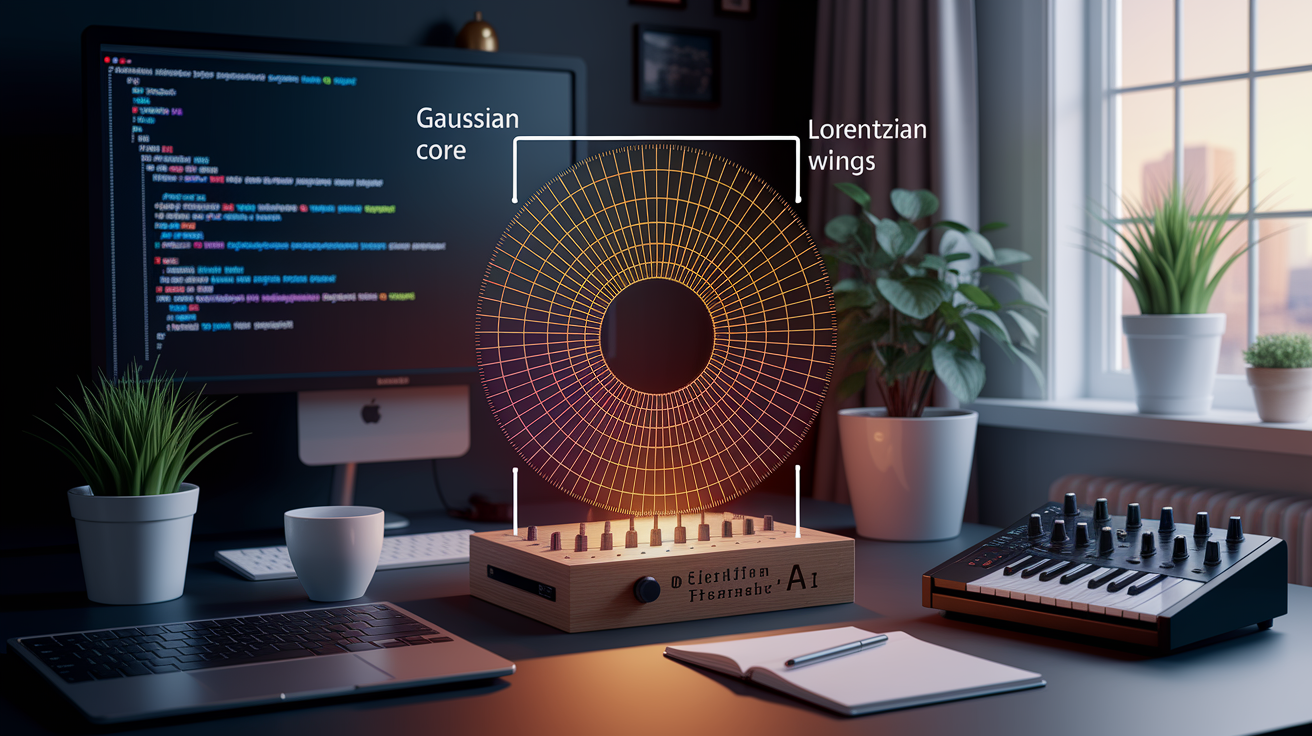
Real stellar lines are shaped by the simultaneous action of multiple broadening mechanisms, each contributing a distinct mathematical form. Thermal and turbulent broadening produce Gaussian profiles. Natural and collisional broadening generate Lorentzian profiles. When both Gaussian and Lorentzian processes operate together (as they almost always do), the result is a Voigt profile, the convolution of a Gaussian core with Lorentzian wings. Voigt profile fitting methods are standard in stellar spectroscopy. Observers measure the widths and depths of observed lines, then fit Voigt functions to extract separate Gaussian and Lorentzian parameters. The Gaussian width encodes temperature and turbulence. The Lorentzian width reflects pressure and natural broadening.
Theoretical broadening models implemented in stellar atmosphere codes (such as MOOG, Spectroscopy Made Easy, or ATLAS) compute synthetic spectra by summing contributions from all active mechanisms. For each line, the code calculates natural, thermal, pressure, and radiative-transfer broadening, then convolves the result with rotational and macroturbulent kernels to match observed profiles. Radiative transfer modeling of line profiles accounts for how photons scatter and absorb as they travel through the atmosphere, coupling line broadening to the temperature and density structure of each atmospheric layer. Matching observed and synthetic profiles allows precise determination of stellar parameters: effective temperature, surface gravity, metallicity, rotation rate, and turbulent velocity.
Analyzing a single line is rarely sufficient. Astronomers fit dozens or hundreds of lines simultaneously to break degeneracies between parameters. Increasing temperature widens lines through thermal Doppler broadening but also changes the ionization balance, shifting which lines are strong. Increasing pressure broadens Lorentzian wings but also affects the continuum level. Only by fitting the full spectrum can these effects be disentangled.
Voigt profile structure:
- Gaussian core: Dominated by thermal Doppler and macroturbulent broadening. Width scales with √(T/M) and turbulent velocity.
- Lorentzian wings: Shaped by collisional and natural broadening. Extend farther from line center, sensitive to pressure and density.
- Voigt mixture: Convolution of Gaussian and Lorentzian. Voigt parameter a (ratio of Lorentzian to Gaussian width) determines profile shape and diagnostic power.
Final Words
We followed how each physical process actually widens a star’s spectral lines — from thermal motions and pressure collisions to rotation and turbulent flows — and how those pieces shape the line core and wings you measure.
We also touched on smaller players (magnetic splitting, quantum lifetimes, molecular bands) and on instrumental smearing, and why observers often fit Voigt-like profiles.
If you ask what causes spectral line broadening in stars, it’s the combined mix of those effects. Understanding them helps astronomers read temperatures, densities, spins, and magnetic fields — and instruments keep getting sharper.
FAQ
Q: What causes the broadening of spectral lines?
A: The broadening of spectral lines is caused by several physical effects: natural (quantum) lifetimes, thermal Doppler motions, pressure or collisional broadening, stellar rotation, macroturbulence, and instrumental resolution.
Q: What causes spectral lines in a star’s light?
A: Spectral lines in a star’s light are produced when atoms or molecules absorb or emit photons at specific energies as electrons change levels, creating dark absorption or bright emission features.
Q: What causes spectral lines in main sequence stars to be broader?
A: Spectral lines in main-sequence stars are broader mainly from higher thermal velocities (thermal Doppler), faster rotation, stronger pressure in dense layers, and convective or macroturbulent velocity fields.