
An astronomical spectrum is a graph that tells you what an object is made of, how hot it is, and whether it’s moving.
Many people think you need a PhD to read spectra, but you don’t.
This clear, step-by-step guide shows how to spot continuous, emission, and absorption patterns, match lines to atoms and molecules, measure redshift, and read line widths.
By the end you’ll know what to check first, how to compare wavelengths and flux, and which features reveal temperature, density, and motion.
Foundations for Understanding an Astronomical Spectrum
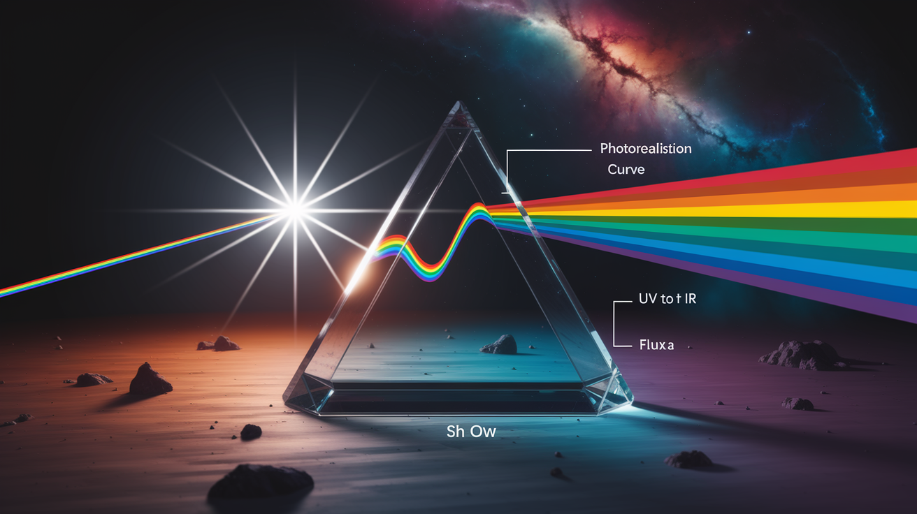
A spectrum is just a graph showing how much light something gives off or soaks up at different wavelengths. The x-axis runs from short wavelengths (ultraviolet on the left) through the colors you can see (violet, blue, green, yellow, orange, red) out to longer wavelengths (infrared on the right). The y-axis tells you brightness at each wavelength, labeled flux, intensity, or counts. Reading one means scanning the graph for patterns, bumps, dips, and shapes that reveal what the object’s made of, how hot it is, and whether it’s coming or going.
Three basic types exist. A continuous spectrum looks smooth, like a hill without breaks. That’s blackbody glow from something dense and hot, like a star’s surface. An emission spectrum shows narrow bright spikes poking up from a dim or flat background. Hot, thin gas (a nebula, say, or the guts of an exploding star) makes those emission lines when electrons drop to lower energy and spit out photons. An absorption spectrum has dark notches cut into an otherwise smooth curve. Cooler gas sitting in front of a hot source eats specific wavelengths, leaving dark lines. Stellar atmospheres do this all the time.
When you crack open a new spectrum, check five things fast:
- Overall shape: smooth? Spiky? Full of dips?
- Big peaks or valleys: emission lines sticking up or absorption cutting down?
- Bright vs. dark lines: above baseline or below?
- Repeating patterns: evenly spaced features often mean a series from one element (hydrogen Balmer lines, for instance).
- Shifted features: known lines at the wrong wavelength? The thing’s moving.
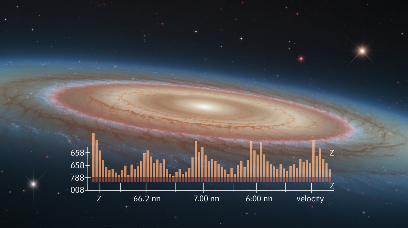
Quick example. Hydrogen’s Balmer-alpha (Hα) emission sits at 656.28 nanometers in a lab at rest. Spot a bright spike near 656 nm in a nebula? That’s hydrogen. Same line closer to 700 nm in a galaxy? It’s redshifted, moving away. Catching these shifts is your first clue to velocity and distance.
Interpreting Wavelength Scales and Flux in an Astronomical Spectrum
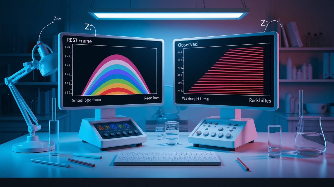
Wavelength units vary. Nanometers (nm) and Ångströms (Å) are most common. One Ångström equals 0.1 nanometers (1 Å = 0.1 nm). The green-yellow part near 550 nm? Same as 5500 Å. Modern spectra usually label the x-axis in nanometers, but older catalogs still use Ångströms. “Rest frame” means the wavelength you’d measure in a lab on Earth. “Observed frame” is what you actually detect from something moving or distant. If a line’s redshifted, its observed wavelength stretches longer than rest. Quick conversion: Hβ listed as 4861.3 Å? Divide by ten to get 486.13 nm.
The y-axis is flux, the amount of light energy you collect per unit time, area, and wavelength. Calibrated spectra give flux in physical units (erg·s⁻¹·cm⁻²·Å⁻¹ or similar). Uncalibrated ones might just show arbitrary detector counts. The continuum is the smooth underlying curve. Emission lines rise above it, absorption lines dip below. Before measuring a line’s real strength, you fit the continuum (often a polynomial or spline) and normalize by dividing observed flux by the fitted continuum. A normalized spectrum sits at baseline 1.0, so it’s easy to see how deep absorption goes or how tall emission peaks. The Sun’s continuous spectrum peaks near 500 nm because its surface runs about 5778 K. Hotter stars peak bluer, cooler ones redder.
Spectral Resolution and Line-Width Reading for Astronomical Spectra
Spectral resolution tells you how finely the spectrum splits neighboring wavelengths. Resolving power is R = λ / Δλ, where λ is the wavelength you’re looking at and Δλ is the smallest difference the instrument can pick out. Higher R, finer detail. Velocity resolution follows roughly Δv ≈ c / R, where c is light speed (~3×10⁵ km/s). R = 10,000 gives Δv ≈ 30 km/s. R = 50,000 yields Δv ≈ 6 km/s. Two features closer than Δv blur into one broad lump.
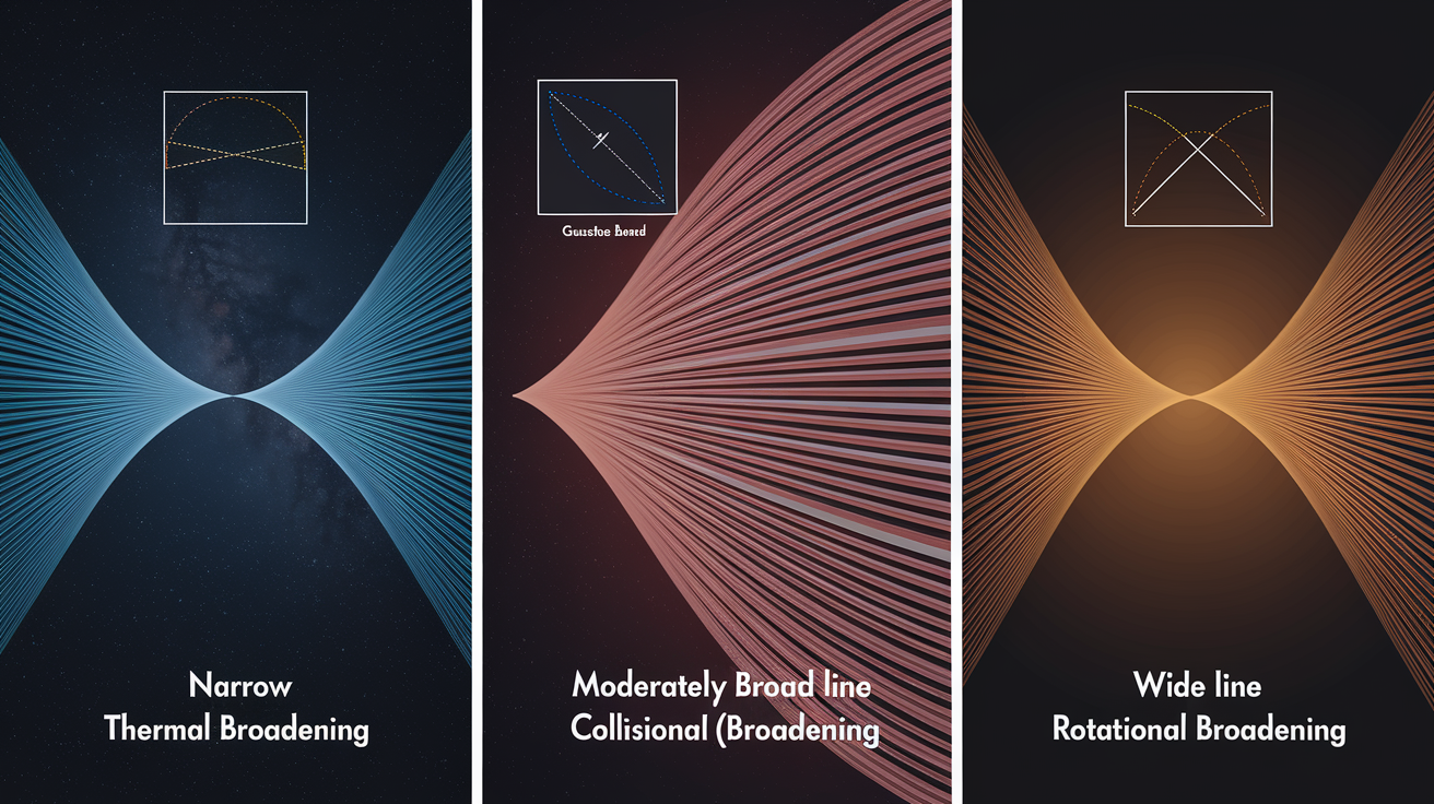
Every line has width, and that comes from physics. Thermal (Doppler) broadening happens because atoms in hot gas zip around randomly. Hotter gas, wider lines. Collisional (pressure) broadening kicks in when atoms bump into each other a lot in dense places, nudging energy levels and smearing the line. Higher density or pressure, more broadening. Rotational broadening shows up in stars or gas that spin. One side moves toward you (blueshift), the other away (redshift), stretching the line across wavelengths. There’s also natural broadening from the Heisenberg Uncertainty Principle: an excited state lasts a short time (typically Δt ≈ 10⁻⁸ seconds), so the energy uncertainty ΔE ties to line-frequency width by Δν ≈ 1/Δt. This intrinsic width is usually tiny compared to the rest. Numeric example: thermal broadening for hydrogen at 10,000 K adds about 0.5 Å (roughly 20 km/s) at Hα, while rotation at 100 km/s can tack on another 1 to 2 Å.
Instrumental broadening comes from the machine itself. Imperfect optics, slit width, detector pixels all blur the line. The instrumental line-spread function (often a Gaussian) has its own width. The observed profile is the true astrophysical profile smeared by this function. If the instrument’s width matches the physical line width, you can’t cleanly separate them. To measure real physical widths (temperature, turbulence, rotation), you need R high enough that instrumental blur is smaller than the signal you’re chasing.
| Line-Broadening Type | Physical Cause | Typical Diagnostic Use |
|---|---|---|
| Thermal (Doppler) | Random thermal motion of atoms | Estimate kinetic temperature of gas |
| Collisional (Pressure) | Frequent collisions in dense gas | Infer density or pressure in stellar atmospheres |
| Rotational | Bulk rotation of star or disk | Measure rotation velocity (v sin i) |
| Natural (Quantum) | Uncertainty principle; finite excited-state lifetime (~10⁻⁸ s) | Usually negligible; sets minimum intrinsic width |
Using Redshift and Doppler Shift When Reading an Astronomical Spectrum
When something moves, its spectral lines shift. Motion away stretches wavelengths toward red (redshift). Motion toward squeezes them blue (blueshift). The redshift parameter is z = (λobs − λrest) / λrest, where λobs is what you measured and λ_rest is the lab value. For slow speeds (non-relativistic), radial velocity is roughly v ≈ c × z, where c is light speed (≈299,792 km/s, or about 3.0×10⁵ km/s). Positive z (and positive v) means receding. Negative z means approaching.
To measure Doppler shift in practice, do this:
- Identify a spectral line in the observed spectrum (bright Hα spike, for instance).
- Compare observed and rest wavelengths: look up rest wavelength (Hα rest = 656.28 nm) and measure where the line actually lands.
- Compute z and v: calculate z = (λ_obs − 656.28) / 656.28, then multiply by c to get velocity in km/s.
Example: you see Hα at 700.0 nm in a distant galaxy. Redshift is z = (700.0 − 656.28) / 656.28 ≈ 0.0666. Velocity is roughly v ≈ 0.0666 × 299,792 km/s ≈ 20,000 km/s, so the galaxy’s racing away at about 20,000 kilometers per second. Measure the same line at 650.0 nm (shorter than rest)? You’d get z ≈ −0.0096 and v ≈ −2,900 km/s, a blueshifted, approaching object. Always use multiple lines when you can. Measuring several hydrogen or metal lines and averaging cuts random errors and confirms you got the ID right.
Identifying Atomic and Molecular Lines Within an Astronomical Spectrum
Every atom, ion, and molecule has its own ladder of energy levels. Transitions between those steps make spectral lines at exact, repeatable wavelengths. To identify a line, you match its observed position (after fixing for redshift) to a catalog of lab rest wavelengths. The rest wavelength is what you measure in a controlled lab with no motion or gravity messing things up. Big online databases (like the NIST Atomic Spectra Database) and printed atlases list thousands of lines for common elements and ions.
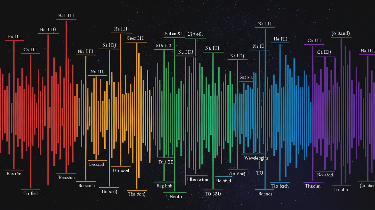
Hydrogen lines are easiest to spot because hydrogen’s everywhere and its lines are strong. The Balmer series (visible range) includes Hα at 656.28 nm (deep red), Hβ at 486.13 nm (blue-green), and Hγ at 434.05 nm (violet). Hotter gas or stronger UV can light up higher series: Lyman-alpha at 121.567 nm lives in the ultraviolet. Metal lines turn up a lot too. Calcium II H and K sit at 393.4 and 396.8 nm (strong absorption in cool stars), and the sodium I D doublet lands at 589.0 and 589.6 nm (that famous yellow pair). Nebulae and ionized-gas zones show forbidden lines (marked with square brackets) from slow, collision-suppressed transitions: [O III] at 495.9 and 500.7 nm (blue-green), [N II] at 654.8 and 658.3 nm (red, flanking Hα), and the [S II] doublet at 6716 and 6731 Å (deep red). Cool stars show broad molecular absorption bands from titanium oxide (TiO) and carbon monoxide (CO), smeared across many wavelengths instead of sharp lines.
Lines you’ll run into all the time:
- Hα (656.28 nm): dominant red emission in H II regions and planetary nebulae; strong absorption in A-type stars.
- Ca II K (393.4 nm): deep absorption in solar-type and cooler stars.
- Na I D (589.0, 589.6 nm): yellow doublet; interstellar absorption and stellar photosphere.
- [O III] 5007 Å (500.7 nm): bright green “nebulium” line in emission nebulae.
- TiO bands (600 to 900 nm): wide, blended absorption in M-type red giants and dwarfs.
- CO bands (near-infrared, 2.3 µm region): molecular signature in very cool stars and brown dwarfs.
Ionization stage (neutral, singly ionized, doubly ionized) changes which lines show. Neutral atoms get Roman numeral I (Na I, Fe I), singly ionized get II (Ca II, Mg II), and so on. Hotter stars show higher ionization because energetic photons strip more electrons. Cooler stars show neutral and low-ionization lines. Matching the ionization pattern helps you peg the star’s temperature and spectral type.
Watch out for blended lines. Two or more so close they merge into one feature. At low resolution, separate lines blur, and you might mistake a blend for a single strong line. Always cross-check with multiple lines of the same element and compare measured wavelengths to high-resolution atlases. If the line width looks weird or asymmetric, suspect a blend or an instrument hiccup.
Measuring Equivalent Widths and Continuum Placement in an Astronomical Spectrum
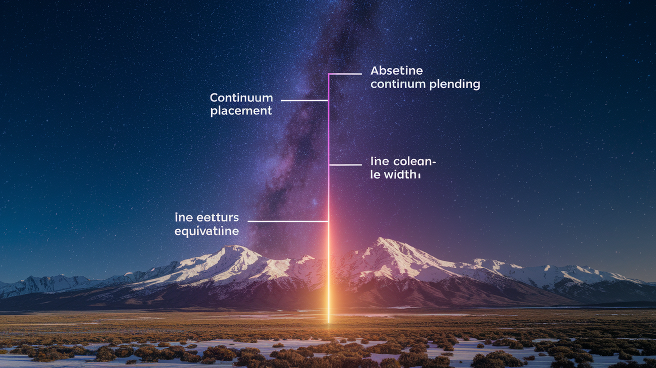
Equivalent width (EW) tells you how strong a line is. For an absorption line, EW is the width (in wavelength units, usually Å or mÅ) of a perfectly black rectangle that eats the same total flux as the real line profile. For an emission line, EW is the width of a rectangle with the same integrated flux above continuum. Math version: EW = ∫ (1 − Fline / Fcontinuum) dλ for absorption (or the integral of excess flux for emission). Bigger EW, stronger line. Typical stellar absorption runs from about 0.1 Å (very weak) to 5 Å (strong metal lines in cool stars). Bright nebular emission (like Hα in an H II region) can hit tens to hundreds of Ångströms.
Three common ways people mess up continuum placement and trash their EW:
- Anchoring continuum on weak absorption: if you fit through shallow lines instead of true line-free spots, you underestimate absorption depth.
- Ignoring curvature: a spectrum’s continuum often slopes or bends because of the star’s temperature and reddening. A straight horizontal fit will be wrong. Use a low-order polynomial or spline.
- Blended lines and pseudo-continuum: in cool stars, thousands of overlapping metal and molecular lines press down a “pseudo-continuum” between the deepest dips. You have to fit locally, not globally, to measure individual line EWs.
When lines are heavily blended (common in high-metallicity or cool stars), define a local pseudo-continuum by connecting nearby windows that are relatively line-free. Measure the EW relative to that local baseline, and note in your analysis that the “continuum” isn’t the true stellar continuum but a practical reference level. Standard practice for late-type stellar abundance work, where clean continuum windows don’t really exist.
Calibrating Astronomical Spectra for Accurate Reading
Before you can interpret anything, you fix raw detector images for instrument quirks. First up is bias and dark subtraction: every CCD or infrared array records a tiny electronic offset (bias) and thermal noise (dark current) even with the shutter closed. Subtract a median-combined bias frame and a scaled dark frame from your science shot to kill these detector ghosts.
Next, flat-fielding corrects pixel-to-pixel sensitivity differences. Each pixel reacts a bit differently to light. Divide your science spectrum by a normalized flat-field frame (an exposure of uniform light) so all pixels report the same count for the same input. Flat-fielding also fixes dust shadows, vignetting, and fringing (interference patterns common in red and near-infrared detectors).
Wavelength calibration maps each pixel along the dispersion to an accurate wavelength. You observe a calibration lamp (often neon, argon, or thorium-argon) that spits out many sharp emission lines at precisely known wavelengths. Identify a dozen or more lamp lines in the spectrum, fit a polynomial that turns pixel number into wavelength, then apply that fit to your science data. Some people also use bright sky emission lines (the O I line at 557.7 nm, for example) as wavelength anchors, especially when arc-lamp coverage is sparse. Calibration errors as small as a fraction of an Ångström can introduce velocity offsets of several km/s, so check residuals carefully.
Sky subtraction and telluric correction remove junk from Earth’s atmosphere. The night sky glows with emission (oxygen, sodium, hydroxyl) and faint continuum. Subtract a sky spectrum (from blank slit regions or a separate sky exposure) to clean your object. Earth’s atmosphere also absorbs light at specific wavelengths. Strong water-vapor bands in red and near-infrared, molecular oxygen (O₂) bands, they create telluric absorption lines. Divide your science spectrum by the spectrum of a hot, featureless standard star observed at similar airmass to scrub these telluric features. After telluric correction, any leftover absorption has to be from your target.
Signal-to-noise ratio (SNR) measures data quality. SNR is signal (counts in continuum or in a line) divided by noise (photon shot noise, detector read noise, sky background). SNR ≥ 10 is the floor for confident line detection. SNR ≥ 30 to 50 is what you want for reliable equivalent-width and radial-velocity measurements. Low SNR hides weak lines and pumps up errors in measured line centers. Always report or estimate your continuum SNR when you publish, because it sets the limit on what you can and can’t detect.
Applying Spectral Diagnostics to Determine Physical Properties

Spectral classification bins stars into types (O, B, A, F, G, K, M) based on absorption-line patterns and strength, which mirror surface temperature. O-type stars (hottest, ~30,000 to 50,000 K) show ionized helium and weak hydrogen. B-type (~10,000 to 30,000 K) display strong neutral helium and growing hydrogen. A-type (~7,500 to 10,000 K) peak in hydrogen Balmer absorption and show ionized metals (Ca II). F, G, K stars (~3,700 to 7,500 K) show neutral and singly ionized metals (Ca II, Na I, Mg I, iron lines) with fading hydrogen. M-type (coolest, <3,700 K) are ruled by molecular bands (TiO, VO) and neutral metal lines. Continuum shape also traces temperature via Wien’s law: λ_max (nm) ≈ 2.898×10⁶ / T(K). A star peaking at 500 nm runs T ≈ 5,800 K (solar-type). One peaking at 250 nm is roughly 11,600 K (hot A or early F).
To measure elemental abundances, you ID lines of a given element, measure their equivalent widths, and compare those EWs to synthetic spectra or curves of growth that account for line-formation physics (excitation, ionization, radiative transfer). A single line’s EW gives a rough abundance guess. Combining many lines of different excitation potentials and ionization stages yields precise, model-dependent abundances. Metallicity ([Fe/H]) is overall metal content relative to the Sun. Stars with [Fe/H] = 0 are solar-metallicity, [Fe/H] = −1 means ten times fewer metals, and [Fe/H] = +0.3 means roughly twice solar. Nebular emission-line diagnostics use ratios of forbidden lines to clock electron temperature and density. The [O III] (λ4959 + λ5007) / λ4363 ratio is temperature-sensitive because the 4363 Å line comes from a higher-energy level. Higher ratios mean lower temperatures. The [S II] λ6716 / λ6731 ratio is density-sensitive: ratio near 1.5 suggests low density (~10² cm⁻³), ratio near 0.5 points to higher density (~10⁴ cm⁻³).
Interstellar absorption features pop up when light from a background star passes through cool gas and dust along the sight line. Common interstellar lines include Na I D, Ca II H and K, and diffuse interstellar bands (DIBs). Broad, shallow absorption at specific wavelengths (5780 Å, 5797 Å, 6284 Å, for instance) with carriers still up for debate, probably big organic molecules. DIBs trace the interstellar medium’s chemistry and can help estimate reddening and distance when you combine them with stellar parameters.
Practical Step-by-Step Guide to Reading an Astronomical Spectrum
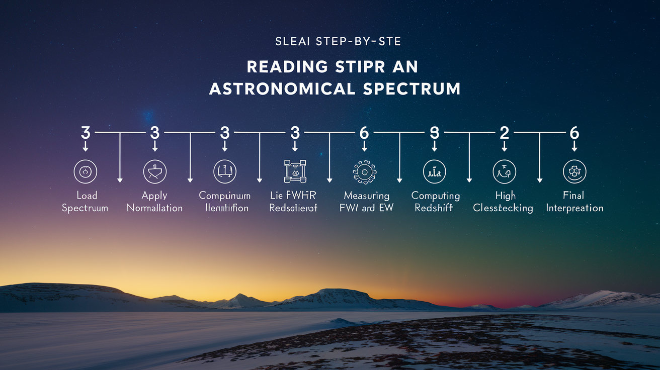
Reading a spectrum mixes calibration, pattern spotting, measurement, and physics. Start with a fully reduced, wavelength and flux calibrated 1D spectrum in hand.
Seven steps to pull the science out:
- Load the calibrated spectrum into analysis software (Python with Astropy/specutils, IDL, or dedicated tools like IRAF, iSpec, or MOOG).
- Inspect continuum and overall shape: fit and normalize the continuum; check for artifacts, cosmic rays, or bad-pixel spikes.
- Identify strong, obvious lines: match their wavelengths to known rest values (use line lists or databases); flag emission vs. absorption.
- Measure line properties: for each ID’d line, record observed central wavelength (λ_obs), full-width at half-maximum (FWHM), and equivalent width.
- Compute redshift and velocities: calculate z = (λobs − λrest)/λ_rest for each line and average to get systemic redshift; convert to radial velocity v ≈ c×z; estimate velocity dispersion from FWHM.
- Cross-check identifications: use multiple lines of the same element to confirm redshift and rule out blends or wrong IDs.
- Apply diagnostics: use line ratios, EWs, and line profiles to infer temperature, density, abundances, rotation, or magnetic fields as fits your science goal.
Difficulty and info you extract depend on spectral resolution. Low-resolution spectra (R ~ 100 to 1,000) are good for broad classification (stellar type, galaxy type), spotting strong emission or absorption, and measuring crude redshifts (±100 km/s or worse). You won’t resolve individual line shapes or nail down precise abundances. High-resolution spectra (R ≥ 20,000 to 50,000) reveal detailed line shapes, velocity structure (rotation, turbulence, outflows), precise radial velocities (a few km/s), and weak lines needed for chemical tagging. At high R you can split closely spaced lines (isotopic shifts, hyperfine structure, or the [S II] doublet, say) and measure magnetic-field splitting (Zeeman effect) when it’s there. Pick your resolution to match your science question: surveys and quick classification use low R; detailed stellar abundances and exoplanet radial velocities demand high R.
Final Words
You’ve already learned to spot a spectrum’s overall shape, pick out emission and absorption features, and notice shifted lines like Hα and Hβ.
We covered reading wavelength and flux axes, spectral resolution and broadening, redshift measurements, line identification and equivalent widths, plus the calibration steps that make those measurements trustworthy.
Practice the step-by-step workflow and the common checks when you try how to read an astronomical spectrum — it becomes clearer with every example, and each spectrum tells a little true story about the cosmos.
FAQ
Q: How to read a light spectrum chart or a star spectrum?
A: Reading a light spectrum chart or a star spectrum means reading wavelength left-to-right, noting overall shape (color/peak), spotting emission or absorption lines, matching line patterns, and checking shifts for motion and redshift.
Q: What are four things a star’s spectrum can tell you?
A: A star’s spectrum can tell you temperature, chemical composition, radial velocity (motion toward or away), and surface properties like gravity or rotation that change line strengths and widths.
Q: What are the 7 types of stars and their meanings?
A: The seven spectral types are O, B, A, F, G, K, M, which indicate temperature and color: O hottest/blue, B very hot, A white, F yellow-white, G (Sun-like) yellow, K orange, M coolest/red.