
Which tells the identity of an atom better: a dark notch or a bright stripe?
Short answer: absorption lines are dark gaps carved out of a continuous rainbow when cooler gas removes specific wavelengths, while emission lines are bright, narrow wavelengths added when excited atoms release photons.
Both are the same atomic fingerprints read in opposite directions.
This post explains how those lines form, how their shapes change with temperature and density, and why astronomers use both to read the chemistry and conditions of stars, nebulae, and lab plasmas.
Core Comparison of Absorption vs Emission Lines in Spectra

Emission lines are bright, narrow wavelengths you get when electrons inside atoms drop from higher energy levels to lower ones, releasing photons at precise frequencies. Absorption lines are dark gaps in a continuous spectrum, formed when electrons absorb specific photons from a background light source and jump to higher energy levels, removing those exact wavelengths from the transmitted beam. Both types work as fingerprints for identifying elements, because the allowed energy jumps are unique to each atom.
Visually, emission lines appear as bright streaks against a dark or continuous background: ---|---|---|--- (bright lines). Absorption lines look like dark notches carved out of a rainbow: ====|==|==== (dark lines interrupting smooth color). A continuous spectrum, such as the light from an incandescent bulb, shows a smooth band of color with no lines at all: ======== (uninterrupted). The key difference is direction. Emission adds light at specific wavelengths, absorption subtracts it.
Stars display absorption lines (called Fraunhofer lines) because their cooler outer layers absorb light from the hotter interior before it reaches us. Gas discharge tubes, neon signs, and glowing nebulae produce emission lines when electric currents or nearby hot stars excite their atoms. Both processes reveal the same chemical fingerprint, just read in opposite directions. One stamps dark, the other stamps bright.
| Feature | Appearance | How It Forms | Typical Source | Background | Example Use |
|---|---|---|---|---|---|
| Emission Line | Bright line at discrete wavelength | Excited electron drops to lower level, emits photon | Hot, low-density gas (neon sign, nebula) | Dark or negligible continuum | Identify elements in emission nebulae |
| Absorption Line | Dark notch in continuous spectrum | Ground-state electron absorbs photon, jumps to higher level | Cool gas in front of hot continuum (stellar atmosphere) | Bright continuous spectrum | Determine stellar composition and temperature |
How Absorption Lines Form in Atoms and Stellar Atmospheres
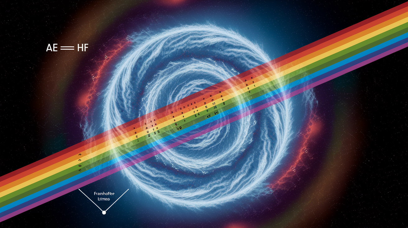
When white light from a hot source passes through a cooler gas, atoms in that gas can absorb photons whose energy exactly matches the difference between two of the atom’s allowed energy levels (ΔE = hf). The electron jumps upward, the photon disappears from the beam, and a dark line appears at that wavelength in the transmitted spectrum. The absorbed photon is later re-emitted, but in a random direction, so the forward beam loses intensity at that frequency. Each element has a unique ladder of energy levels, so each produces its own set of dark lines.
Stellar atmospheres are textbook examples. Deep inside a star, high temperature and density generate a smooth, continuous rainbow (blackbody spectrum). As that light travels outward through cooler, lower-density layers near the surface, atoms in those layers absorb photons at their characteristic wavelengths. By the time the light reaches Earth, thousands of dark Fraunhofer lines are stamped across the spectrum. Each one revealing which elements are present in the star’s outer envelope and how tightly packed or fast-moving those atoms are (affecting line width and position).
Photon removal: Specific wavelengths are subtracted from the continuous beam.
Electron excitation: Ground-state or low-lying electrons absorb energy and move to higher states.
Isotropic re-emission: The absorbed photon is eventually re-radiated in a random direction, not necessarily back along the line of sight.
Net dimming: Along the observer’s line of sight, the intensity at the absorbed wavelength drops, creating a dark line.
How Emission Lines Form in Hot Gas, Nebulae, and Laboratory Tubes

Emission lines appear when electrons in excited states drop to lower energy levels, releasing photons at precise wavelengths determined by ΔE = hf. The excitation can come from collisions with other particles, absorption of ultraviolet light from nearby hot stars, or electric currents running through low-pressure gas. Each downward jump emits one photon. Because the energy levels are quantized, the emitted light clusters into narrow, bright lines rather than spreading across the spectrum.
Gas discharge tubes, such as neon signs and laboratory spectrum lamps, demonstrate emission directly. An electric field accelerates electrons through a low-pressure gas, and when those fast electrons collide with atoms, they knock orbital electrons into higher states. Those excited electrons quickly fall back down, emitting colored light at wavelengths unique to the gas inside the tube. Neon glows red-orange. Hydrogen produces a set of four visible lines including the famous red H-alpha at 656 nm. Mercury and argon add their own signatures. The result is a spectrum of bright lines on a dark background.
Emission nebulae work on a larger scale. Ultraviolet photons from young, hot stars ionize hydrogen and other gases in nearby clouds. When free electrons recombine with ions, they cascade down through energy levels, emitting photons at each step. Collisions in the hot gas also excite atoms directly. The most prominent nebular lines are H-alpha (red), [O III] at 496 and 501 nm (green), and [N II] near H-alpha (also red). These recombination and collisionally excited lines tell astronomers the nebula’s temperature, density, and chemical makeup.
Quantum Transitions Behind Absorption and Emission Line Spectra

Atoms hold electrons in discrete energy levels, like rungs on a ladder. An electron can only sit on a rung, never between them. The ground state is the lowest rung. Excited states are higher rungs. Moving between rungs requires absorbing or emitting a photon whose energy exactly matches the gap: ΔE = Eupper − Elower = hf, where h is Planck’s constant and f is the photon’s frequency. If the energy doesn’t match, the photon passes by without interacting.
Quantum mechanics also enforces selection rules, mathematical constraints that allow some transitions and forbid others. Permitted transitions are efficient and produce strong lines. Forbidden transitions break one of the usual rules (such as a change in electron spin or orbital angular momentum) and are much slower, but they can still occur in low-density nebulae where atoms wait a long time between collisions. Forbidden lines are labeled with square brackets, for example [O III]. Fluorescence is a cascade process: an atom absorbs a high-energy photon (often ultraviolet), jumps to a high level, then cascades down through intermediate levels, emitting multiple lower-energy photons. Turning one UV photon into several visible or infrared ones.
Energy-Level Structures
Every element has a unique pattern of allowed energy states. Hydrogen, with one electron, has a simple ladder given by E_n = −13.6 / n² eV (n = 1 is ground state, n = 2 is first excited, and so on). Heavier elements have many electrons and correspondingly more complex level diagrams, but the principle is the same: transitions between fixed rungs produce photons at fixed wavelengths. Because wavelength λ = c / f, each ΔE maps to a unique color. That one-to-one link between atomic structure and wavelength is why spectral lines act as chemical fingerprints. Oxygen’s ladder is different from iron’s, so their line sets never overlap exactly.
Spectral Line Profiles and Broadening Effects
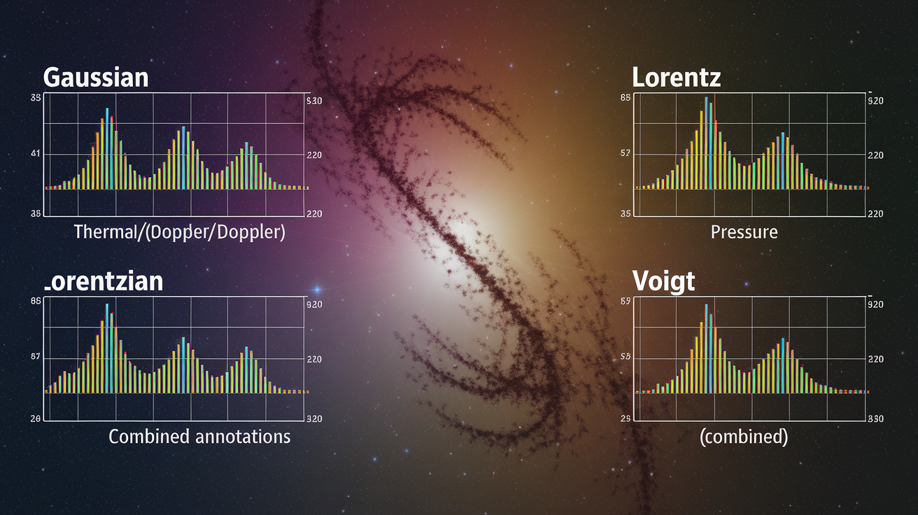
Real spectral lines aren’t infinitely narrow spikes. They have a measurable width and shape called the line profile. Three main physical processes broaden lines. Thermal (Doppler) broadening arises because atoms in a hot gas move randomly in all directions. Atoms moving toward the observer emit light that’s slightly blue-shifted, atoms moving away emit red-shifted light, and the combined result is a Gaussian-shaped line centered on the rest wavelength. Hotter gas means faster atoms and broader lines. Pressure (collisional) broadening happens when atoms are packed close enough that collisions interrupt the emission or absorption process, shortening the photon’s effective wavelength uncertainty and widening the line into a Lorentzian profile. Natural (lifetime) broadening is a quantum effect. Excited states have finite lifetimes, and Heisenberg’s uncertainty principle (ΔE Δt ≈ ħ) means a short-lived state has inherent energy uncertainty, spreading the line even in a perfectly still, isolated atom.
In practice, all three effects combine. The Voigt profile is the convolution of Gaussian (thermal) and Lorentzian (pressure and natural) shapes and is the standard model for fitting observed lines. Measuring the width and shape of a line reveals the gas temperature (from Doppler width), density (from collisional width), and sometimes rotation or turbulence (from extra Doppler shifts).
| Broadening Type | Cause | Profile Shape | Typical Environment |
|---|---|---|---|
| Thermal (Doppler) | Random atomic velocities | Gaussian | Hot stars, nebulae |
| Pressure (Collisional) | Frequent atom–atom collisions | Lorentzian | Dense stellar atmospheres, lab arcs |
| Natural (Lifetime) | Heisenberg uncertainty in short-lived states | Lorentzian | All atoms (usually smallest effect) |
| Combined | All three mechanisms together | Voigt | Most observed spectra |
Real Astronomical Examples of Absorption and Emission Lines
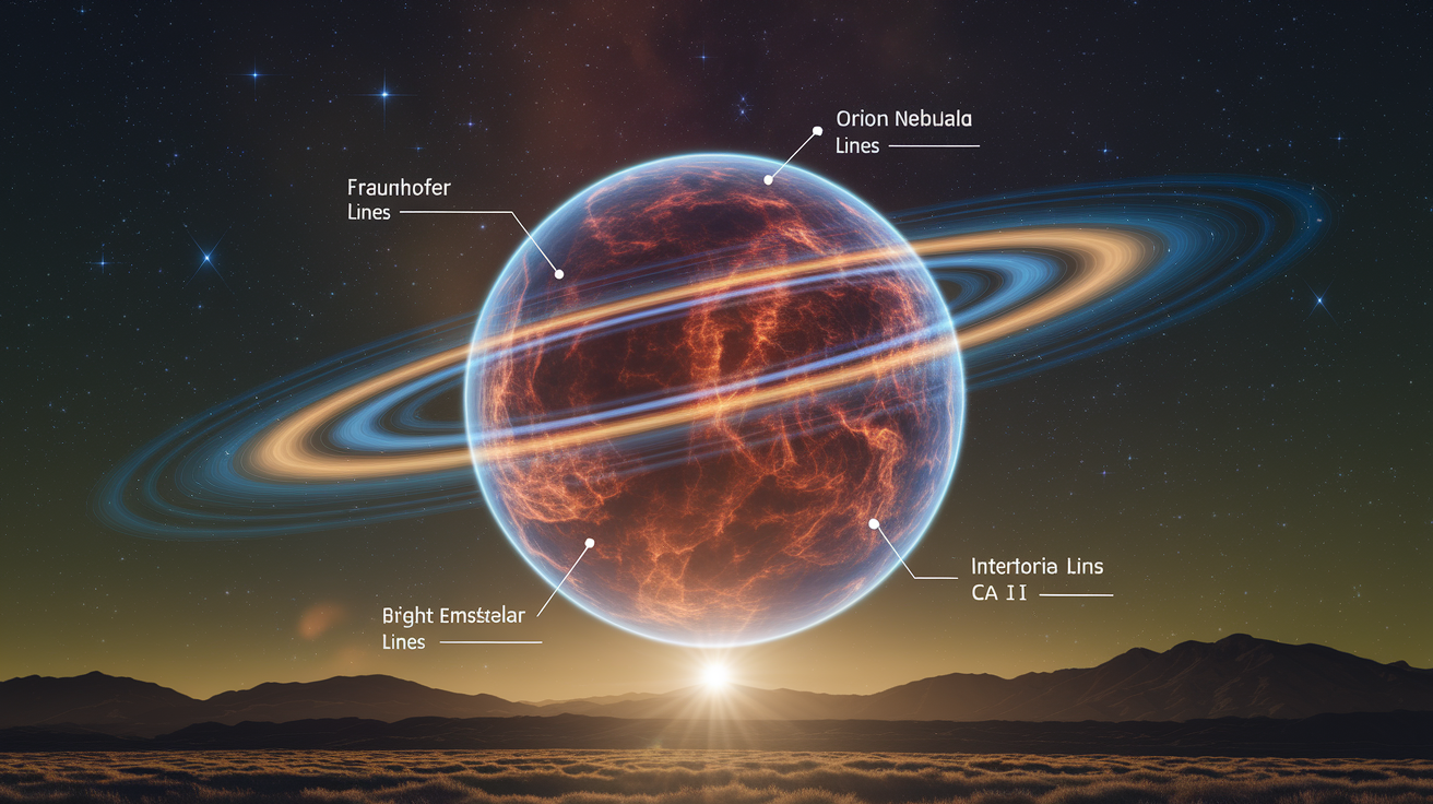
The first detailed catalog of solar absorption lines was compiled by Joseph von Fraunhofer in the early 1800s. The strongest dark lines in the Sun’s spectrum still carry letter names (the D lines are sodium, H and K are ionized calcium). Fraunhofer’s work showed that the Sun isn’t a featureless glowing ball but a layered atmosphere full of identifiable elements. Later, the same lines were found in other stars, enabling the first chemical surveys of the universe.
Emission nebulae, clouds of gas ionized by nearby hot stars, display bright lines instead of dark ones. The red glow of the Orion Nebula comes mostly from H-alpha at 656 nm. Green-tinted nebulae owe their color to doubly ionized oxygen, [O III], emitting at 496 and 501 nm. The [N II] doublet near 658 nm adds to the red. The [S II] doublet near 672 nm is used as a density diagnostic. Its intensity ratio shifts with electron density. Planetary nebulae, supernova remnants, and H II regions all show strong emission-line spectra, each revealing temperature, density, and abundances through line strengths and ratios.
Interstellar absorption features appear when light from a distant star passes through cold gas clouds between the star and Earth. Narrow absorption lines from neutral sodium (Na D doublet at 589.0 and 589.6 nm) and singly ionized calcium (Ca II H and K at 393.4 and 396.8 nm) mark the presence of diffuse interstellar medium. These lines are often much narrower than the stellar lines because the interstellar gas is cold and low-density. Galaxy spectra also split into two broad classes: emission-line galaxies, dominated by star-forming regions with bright H-alpha and [O III], and absorption-line galaxies, where old stellar populations produce deep metal absorption lines and little ongoing star formation.
Solar Fraunhofer lines: thousands of absorption features identifying elements in the Sun’s photosphere.
H-alpha emission at 656 nm: hallmark of ionized hydrogen in nebulae and star-forming galaxies.
[O III] doublet at 496, 501 nm: green nebular emission from hot, low-density gas.
Na D interstellar absorption: cold neutral gas clouds along the line of sight to distant stars.
Ca II H and K absorption: strong interstellar and stellar features used to trace gas and stellar populations.
Using Line Spectra in Astronomy: Composition, Redshift, and Diagnostics

Every element imprints a unique barcode of lines, so identifying which lines appear immediately tells you which elements are present. Measuring the relative strengths of lines from the same element (for example, the Balmer series of hydrogen) reveals the gas temperature, because higher temperatures populate higher energy levels and change the intensity ratios. Comparing lines from different ionization states (neutral vs singly ionized vs doubly ionized) constrains both temperature and the ionizing radiation field.
Doppler shifts move spectral lines. If a star or galaxy is moving toward Earth, all its lines shift to shorter (bluer) wavelengths. Motion away shifts them to longer (redder) wavelengths. The fractional shift Δλ / λ₀ equals the radial velocity divided by the speed of light (non-relativistic case). Astronomers measure the wavelength of a known line (such as H-alpha at 656.3 nm in the lab), compare it to the observed wavelength, and compute the velocity. For distant galaxies, cosmological redshift stretches wavelengths as the universe expands. Measuring the redshift of familiar lines like H-alpha or [O III] yields the galaxy’s distance and lookback time.
Abundance determination goes beyond presence/absence. The strength of an absorption or emission line depends on how many atoms of that element are available, the temperature, the density, and the optical depth of the gas. Stellar abundance analysis uses grids of synthetic spectra (model atmospheres) to match observed line depths, yielding the mass fraction of iron, carbon, oxygen, and dozens of other elements. These measurements trace the chemical history of stars and galaxies, showing how supernovae and stellar winds enrich the interstellar medium over time.
Nebular diagnostics exploit line ratios that are sensitive to physical conditions but nearly independent of abundance. The [O III] λ5007 / H-beta ratio is a temperature indicator. The [S II] λ6716 / λ6731 ratio varies with electron density. Collisions preferentially depopulate the upper level of one line, so measuring the ratio pins down how often atoms collide, which directly gives the number of particles per cubic centimeter. The [N II] / H-alpha ratio helps distinguish star-forming regions (low ratio) from active galactic nuclei (high ratio). These diagnostics turn spectra into thermometers, barometers, and chemical assay kits for objects millions of light-years away.
Hydrogen as the Key Model: Balmer, Lyman, and Worked Photon Examples
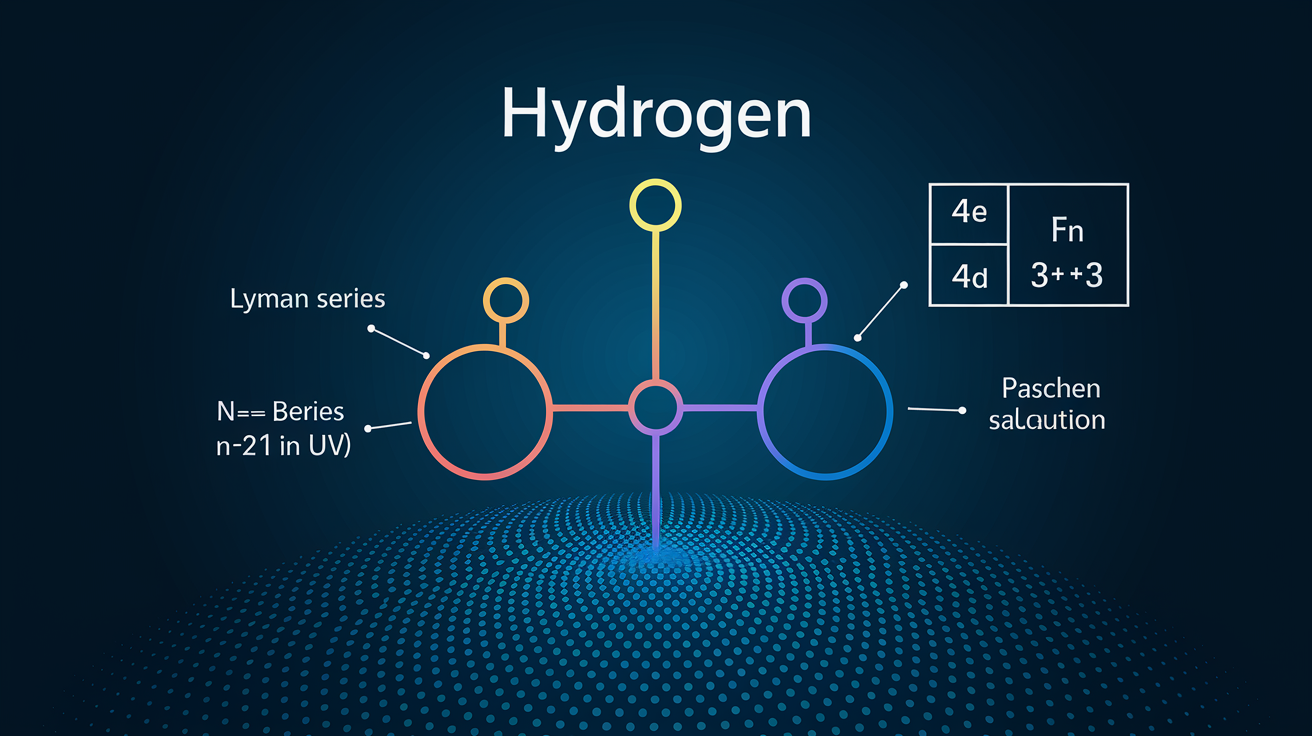
Hydrogen is the simplest atom, one proton, one electron, so its energy levels follow the clean formula E_n = −13.6 / n² eV. Transitions down to the ground state (n = 1) produce the Lyman series in the ultraviolet. The strongest, Lyman-alpha (n = 2 → 1), sits at 121.6 nm. Because Earth’s atmosphere blocks UV, Lyman lines are observed from space telescopes or inferred from absorption in distant quasar spectra. Transitions down to n = 2 form the Balmer series, which falls in the visible and near-UV: H-alpha (656.3 nm, red), H-beta (486.1 nm, cyan), H-gamma (434.0 nm, blue-violet), and H-delta (410.2 nm, violet). The Balmer lines dominate the spectra of hot stars and emission nebulae. Transitions to n = 3 and higher (Paschen, Brackett, Pfund) lie in the infrared and are important for cool stars and dusty regions.
A worked example shows the mechanics. Take the n = 2 → 1 transition (Lyman-alpha). The energies are E₁ = −13.6 eV and E₂ = −13.6 / 4 = −3.4 eV, so ΔE = E₂ − E₁ = 10.2 eV. The photon frequency is f = E / h = 10.2 eV / (4.136×10⁻¹⁵ eV·s) = 2.466×10¹⁵ Hz. The wavelength is λ = c / f = (3.0×10⁸ m/s) / (2.466×10¹⁵ Hz) = 1.217×10⁻⁷ m = 121.7 nm, firmly in the ultraviolet range (visible light spans roughly 400–700 nm). For the n = 3 → 1 transition, E₃ = −13.6 / 9 = −1.51 eV, so ΔE = 12.09 eV, f ≈ 2.92×10¹⁵ Hz, and λ ≈ 102.6 nm. Shorter and more energetic than Lyman-alpha.
| Series | Typical Wavelength Range | Example Transition |
|---|---|---|
| Lyman | 91–122 nm (far-UV) | n = 2 → 1 (Lyman-alpha, 121.6 nm) |
| Balmer | 365–656 nm (visible and near-UV) | n = 3 → 2 (H-alpha, 656.3 nm) |
| Paschen | 820–1875 nm (near-IR) | n = 4 → 3 (1282 nm) |
Observational Challenges: Telluric Absorption, Sky Emission, and Spectral Resolution
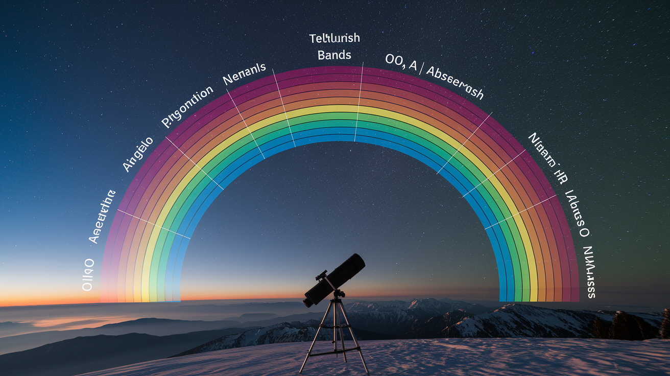
Earth’s atmosphere adds its own absorption and emission features, collectively called telluric lines. Molecular oxygen, water vapor, and ozone carve broad absorption bands in the red and infrared (the A- and B-bands of O₂ near 760 and 687 nm, water bands in the near-IR). These atmospheric lines can overlap astronomical lines, making it hard to measure the true shape and depth. Astronomers correct for telluric absorption by observing bright standard stars at similar airmass and dividing the target spectrum by the standard, or by using atmospheric transmission models.
The night sky isn’t perfectly dark. It glows faintly with emission lines from airglow (oxygen and hydroxyl) and scattered moonlight or zodiacal light. The brightest sky lines are [O I] at 557.7 and 630.0 nm and the OH bands in the near-IR. When taking a long-exposure spectrum, sky emission adds a constant offset. Observers subtract it by recording nearby blank sky in a separate slit position or fiber, then subtracting that sky spectrum from the target. Imperfect subtraction leaves residual spikes that can mimic weak astronomical features.
Spectral resolution R = λ / Δλ measures how finely a spectrograph can distinguish neighboring wavelengths. Low-resolution spectrographs (R ~ 100–1000) blur lines together but collect light efficiently, useful for faint targets. Medium-resolution instruments (R ~ 5000–20,000) separate most emission and absorption lines clearly. High-resolution spectrographs (R > 30,000) resolve line profiles, revealing Doppler broadening, velocity structure, and closely spaced multiplets. The choice of resolution is a trade-off: higher R means dimmer spectra and longer exposures, but it unlocks fine details that low-R data can’t reach.
Oxygen and water absorption bands: atmospheric telluric features that contaminate ground-based spectra in the red and infrared.
Airglow emission lines: faint sky glow from [O I] and OH that must be subtracted from target spectra.
Spectral resolution limits: low R blurs lines together; high R separates them but requires brighter targets or longer integrations.
Airmass dependence: telluric strength increases when observing near the horizon, where light passes through more atmosphere.
Identifying Spectral Lines: Databases, Line Lists, and Practical Tips

Once you have a spectrum, the next step is matching the observed wavelengths to known atomic and molecular transitions. Atomic line lists compiled by laboratories and theorists catalog hundreds of thousands of lines, including rest wavelength, element and ionization state, transition probabilities, and energy levels. The Kurucz line list and the NIST Atomic Spectra Database are two widely used references. For molecules, databases like HITRAN (for Earth atmosphere) and ExoMol (for exoplanet and stellar atmospheres) provide transition data.
Calibration lamps provide wavelength standards. Before or after each observation, astronomers expose the spectrograph to light from gas discharge lamps filled with thorium-argon, neon, or xenium. These lamps produce dense forests of sharp emission lines at precisely known wavelengths. By fitting a polynomial or spline to the lamp spectrum (pixel position vs wavelength), the instrument’s wavelength solution is determined. Any drift or distortion in the optics or detector is mapped out and corrected. Without calibration, even strong lines can be misidentified because the raw detector pixel numbers don’t directly correspond to wavelengths.
Line identification starts with the brightest, most isolated features. In visible spectra of hot stars, the Balmer lines stand out. In nebulae, H-alpha and [O III] are unmistakable. Weaker lines require careful comparison to catalogs and cross-checks with expected line ratios (for example, the [O III] doublet should always have the 5007 line roughly three times stronger than 4959). Redshift or blueshift is applied first. Once the velocity is known, all lines shift together, so finding one strong line pins down the rest. Automated pipelines use pattern-matching algorithms, but visual inspection remains essential to catch blends, cosmic rays, and artifacts.
Tools and Reference Standards
Laboratory spectroscopy anchors astronomical line identification. Physicists measure emission and absorption wavelengths in controlled conditions, known gas, known temperature, known pressure, and publish the results as reference atlases. The solar spectrum itself serves as a secondary standard, because Fraunhofer lines are so well measured that their wavelengths are often used to calibrate echelle spectrographs. Calibration lamps built into telescopes and instruments ensure that each night’s data can be traced back to these fundamental standards, maintaining sub-angstrom wavelength accuracy even as temperature and mechanical flexure shift the optics. This chain of reference, from lab to lamp to star, makes it possible to identify a faint iron line in a distant galaxy’s spectrum with confidence.
Final Words
We dove straight into how absorption and emission lines form and how they differ in appearance.
You saw the quantum step: electrons absorb exact-energy photons to make dark absorption lines, and falling electrons release photons to make bright emission lines. We used ASCII diagrams, lab tubes, and stellar Fraunhofer lines to make it concrete.
If one thing sticks, let it be this: absorption line vs emission line explained. Dark lines mean photons were removed; bright lines mean photons were added. Now you can read spectra with more confidence.
FAQ
Q: What is the difference between absorption and emission lines, absorbed versus emitted light, and energy absorption versus emission?
A: The difference is that absorption removes photons when electrons jump to higher energy levels, producing dark lines, while emission releases photons when electrons fall to lower levels, producing bright lines.
Q: What can emission and absorption lines tell us?
A: Emission and absorption lines tell us which elements are present, plus temperature, density, and motion; wavelengths identify atoms, strengths give abundances or conditions, and Doppler shifts measure velocity.