
How can a satellite hundreds of miles up spot a new wildfire or a failing crop?
By circling Earth and using sensors that read reflected light, emitted heat, or radar echoes.
Sensors are instruments that convert those signals into data.
Orbit altitude and path, from low Earth orbit (LEO, a few hundred kilometers) to geostationary far above, set how sharp the view is and how often a spot is revisited.
This post explains the sensors, orbits, data flow, and why those parts matter for maps, weather, and disaster response.
Core Mechanisms Behind Earth Observation Satellite Operations
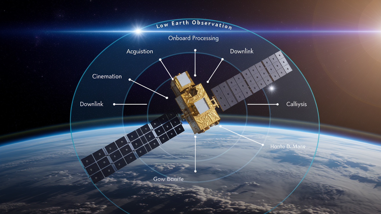
Earth observation satellites work by circling the planet with sensors that measure reflected sunlight, heat radiating from the surface, or echoes bouncing back from radar and laser pulses. Most fly in Low Earth Orbit, somewhere between 200 and 2,000 kilometers up, where they can grab high-resolution details and pass over the same spot multiple times a day. Others sit way out in Geostationary Orbit at roughly 35,786 kilometers, locked over one hemisphere so they can watch weather systems unfold in real time. Altitude shapes everything: what the satellite sees, how sharp the image looks, how often it comes back.
Sensors split into two groups. Passive optical systems record visible, near-infrared, and shortwave infrared light bouncing off forests, cities, oceans. Think of them as cameras shooting pictures in sunlight. Thermal infrared sensors catch heat radiating up from the ground or sea, revealing surface temperatures and volcanic hot spots. Active systems send out their own signals. Synthetic Aperture Radar emits microwave pulses and times the echoes to map terrain through clouds and darkness. LiDAR fires laser beams to measure precise heights and build elevation models. Once the sensor collects raw measurements, onboard electronics convert analog signals into digital data, apply initial calibration, and store the imagery in memory until the satellite flies within range of a ground station.
Data reaches Earth via radio downlink, usually X-band or Ka-band for high-speed image transfer and S-band for telemetry and commands. Ground stations receive the transmission, check integrity, and route files to processing centers. Specialists there correct for atmospheric distortion, align pixels to geographic coordinates, stitch overlapping frames into seamless maps. Advanced algorithms calculate vegetation indices, classify land cover, detect changes between dates, and generate products like orthomosaics, digital elevation models, contour maps. The complete workflow unfolds in five steps:
- Acquisition – Sensors record raw radiance values, radar returns, or laser pulses across a ground swath.
- Onboard processing – Electronics digitize signals, compress files, store data in memory.
- Downlink – The satellite transmits imagery and telemetry to a ground station when in view.
- Calibration and correction – Processors apply radiometric calibration, geometric correction, atmospheric adjustments.
- Analysis and product generation – Mosaicking, index calculation, classification, change detection produce final maps and datasets.
Orbit Types That Enable Earth Observation Performance
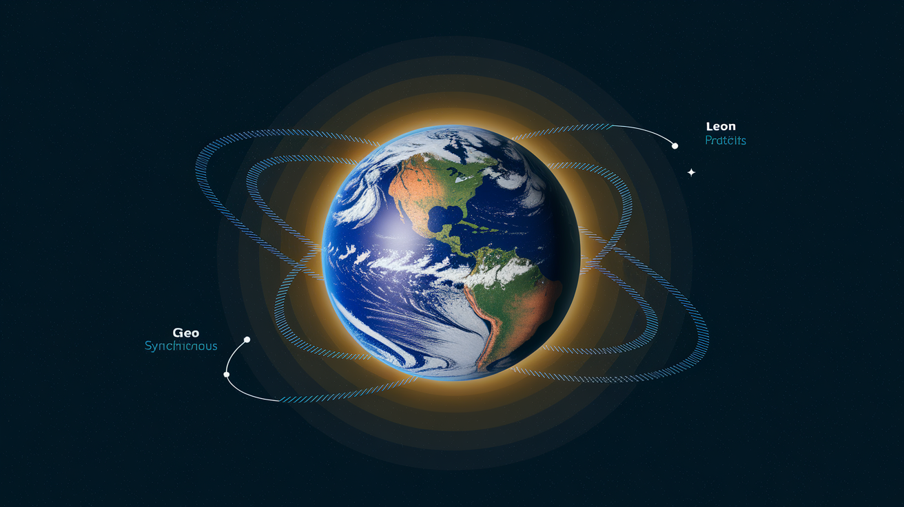
Orbit altitude and geometry determine how much of Earth a satellite sees, how often it returns, how fine the details appear. Low Earth Orbit places spacecraft between roughly 200 and 2,000 kilometers, where closer proximity delivers sharper images and wider ground coverage with each pass. Many LEO satellites follow polar or sun-synchronous paths, circling over both poles and crossing the equator at the same local solar time each day. Consistent lighting, simpler change detection, global reach within days. The Landsat series pioneered sun-synchronous imaging back in the 1970s and still operates today with new generations capturing 15 to 30 meter resolution scenes every 16 days.
Geostationary Orbit sits at 35,786 kilometers directly above the equator, where orbital velocity matches Earth’s rotation and the satellite appears stationary over one point. GEO platforms monitor entire hemispheres continuously, perfect for weather tracking and early warning of storms. The tradeoff? Distance. Features that LEO satellites resolve in meters blur to kilometers from GEO. Quick comparison:
LEO (200–2,000 km) – High spatial resolution, frequent global passes, short revisit times. Used for land mapping and detailed resource monitoring.
GEO (~35,786 km) – Fixed view of one hemisphere, continuous imaging, coarse resolution. Used for weather and communications.
Polar orbits – Pass over both poles, cover the entire planet, useful for climate and ice monitoring.
Sun-synchronous orbits – Cross the equator at the same local time, provide consistent lighting, essential for long-term change detection.
Sensor Technologies Used in Earth Observation
Passive Optical and Multispectral Sensors
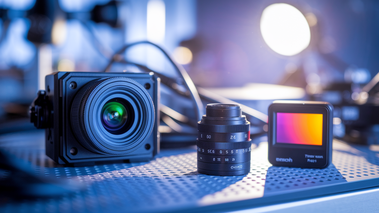
Passive optical sensors collect sunlight reflected from Earth’s surface across several wavelength bands. Typically visible red, green, blue plus near-infrared and shortwave infrared. By separating light into discrete channels, these multispectral imagers reveal features invisible to the naked eye. Healthy vegetation reflects strongly in near-infrared, water absorbs it, bare soil shows unique patterns in shortwave bands. The data enable land-cover classification, crop health assessment, urban mapping. High-resolution commercial satellites and many national systems capture sub-meter to 30 meter pixels, balancing detail against swath width and revisit frequency.
Hyperspectral and Thermal Infrared Sensors
Hyperspectral sensors extend multispectral imaging by recording hundreds of narrow, contiguous wavelength bands, creating a complete spectrum for every pixel. Fine spectral resolution identifies specific minerals, detects subtle vegetation stress, maps pollutants that broader bands would miss. Thermal infrared sensors measure heat emitted by the surface, longer wavelengths around 8 to 14 micrometers, rather than reflected sunlight. Day or night, they produce temperature maps that highlight volcanic hot spots, forest fires, urban heat islands, sea-surface temperature patterns critical for weather forecasting and climate research.
Active Radar (SAR) Systems
Synthetic Aperture Radar operates by transmitting microwave pulses toward the ground and measuring the strength and timing of the echoes that bounce back. Because it supplies its own illumination, SAR works through clouds, rain, smoke, darkness. Conditions that blind optical sensors. The backscatter signal encodes surface roughness, moisture, structure. Calm water appears dark, rough seas or forests scatter strongly, metallic objects return bright spikes. Interferometric SAR compares two radar images taken from slightly different positions or times to detect millimeter-scale ground motion, map elevation, monitor subsidence, landslides, infrastructure deformation. This all-weather, day-night capability makes SAR indispensable for disaster response, oil-spill detection, monitoring remote regions where cloud cover persists.
LiDAR and Microwave Altimetry
Light Detection and Ranging fires rapid laser pulses, often hundreds of thousands per second, and times each return to measure distance with centimeter precision. From orbit, LiDAR builds digital elevation models, maps forest canopy height, tracks ice-sheet thickness. Microwave altimeters work similarly but use radar pulses to measure ocean height, lake levels, ice topography over large footprints. Both techniques convert time-of-flight data into three-dimensional point clouds or gridded elevation products that support hydrology, forestry biomass estimates, glaciology.
How Satellites Capture, Process, and Transmit Earth Imagery

Imaging begins when the sensor’s field of view sweeps across the target area and detectors convert incoming photons, radar echoes, or laser returns into electrical signals. The complete chain from acquisition to final map product proceeds in six steps:
- Raw acquisition – Sensors record radiance values, backscatter amplitudes, or pulse travel times across a swath, building a two-dimensional array of measurements.
- Digitization and onboard calibration – Analog signals are converted to digital numbers. Onboard processors apply gain and offset corrections, compress files to reduce bandwidth, tag each frame with time and orbit metadata.
- Temporary storage – Data reside in solid-state memory until the satellite passes over a ground station or relay satellite with line-of-sight communication.
- Downlink – The spacecraft transmits imagery via X-band or Ka-band radio links, delivering gigabits per second for high-resolution data, and sends telemetry and commands over S-band or UHF channels.
- Ground-station reception – Antennas receive the signal, demodulate the stream, verify checksums, forward files to mission processing centers.
- Processing and product generation – Specialists perform radiometric calibration to convert digital counts into physical units like reflectance or temperature, geometric correction to align pixels with a map grid, atmospheric correction to remove haze and scattering, mosaicking to stitch adjacent frames. Advanced algorithms then compute vegetation indices, classify land cover, detect changes, generate orthomosaics, digital elevation models, contour maps ready for analysis.
A simplified summary of key processing stages:
| Processing Step | Purpose |
|---|---|
| Radiometric calibration | Convert sensor counts to reflectance or radiance |
| Geometric correction | Align pixels to a coordinate system and correct distortion |
| Atmospheric correction | Remove scattering and absorption effects to reveal true surface properties |
Resolution, Swath Width, and Revisit Time Fundamentals
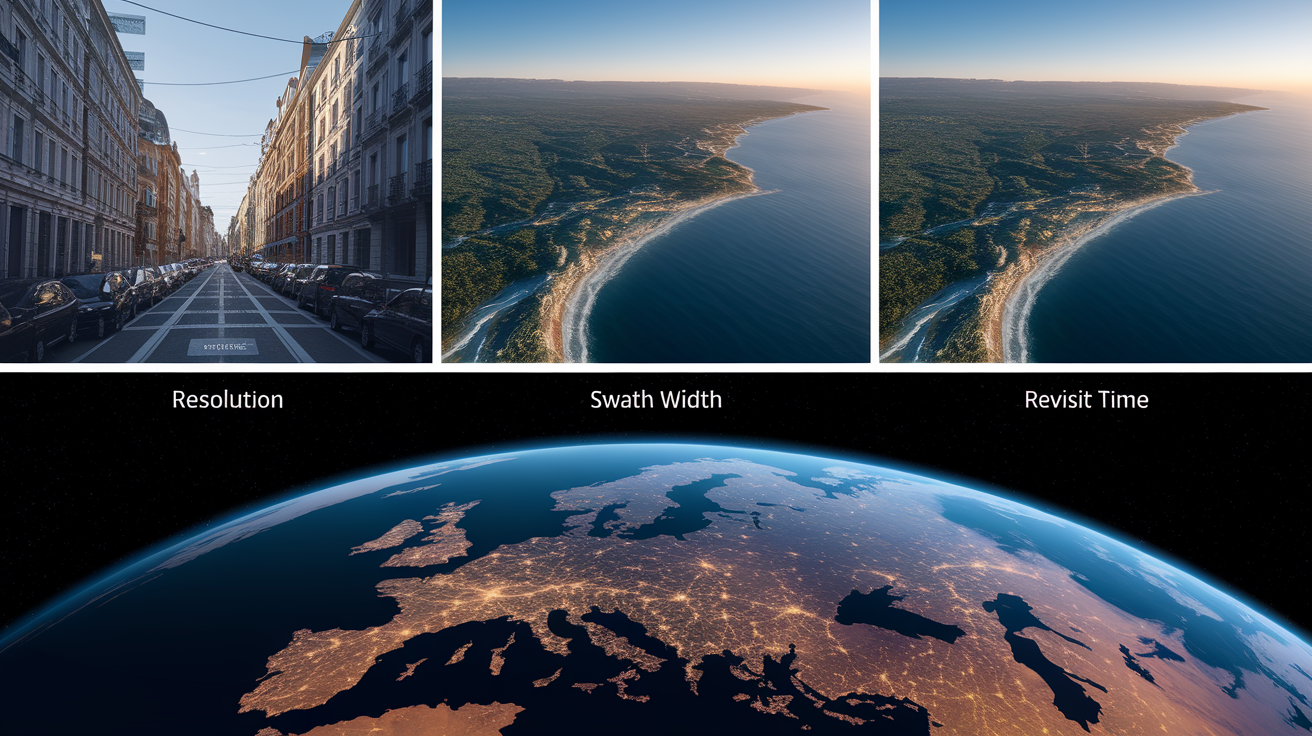
Resolution describes how finely a satellite can distinguish details and comes in four types. Spatial resolution is the ground size of a single pixel. Finer resolution reveals smaller objects but narrows the swath width and requires more data. Spectral resolution counts how many wavelength bands the sensor records and how narrow each band is. More bands enable precise material identification. Temporal resolution measures how often the satellite returns to the same location. Daily revisit supports rapid change detection, while weekly or monthly passes suffice for seasonal monitoring. Radiometric resolution defines how many brightness levels the sensor can distinguish, typically expressed in bits per pixel. Higher bit depth captures subtle contrasts in shadow or bright surfaces.
These parameters interact through design tradeoffs. A satellite in low orbit achieves fine spatial resolution but covers a narrow swath, so reaching global coverage takes many orbits. Widening the swath or lowering altitude shortens revisit time but may degrade pixel size. Geostationary platforms offer continuous hemispheric views but sacrifice spatial detail. Real-world effects:
Sub-meter resolution – Identifies individual vehicles, building outlines, small agricultural plots. Used in urban planning and precision agriculture.
10 to 30 meters – Maps land cover, forest patches, large infrastructure. Common in free global datasets like Landsat and Sentinel.
Multispectral (3–10 bands) – Sufficient for vegetation indices and basic classification.
Hyperspectral (hundreds of bands) – Resolves mineral types, crop diseases, pollution signatures invisible to broader sensors.
Environmental and Climate Insights Derived From EO Data
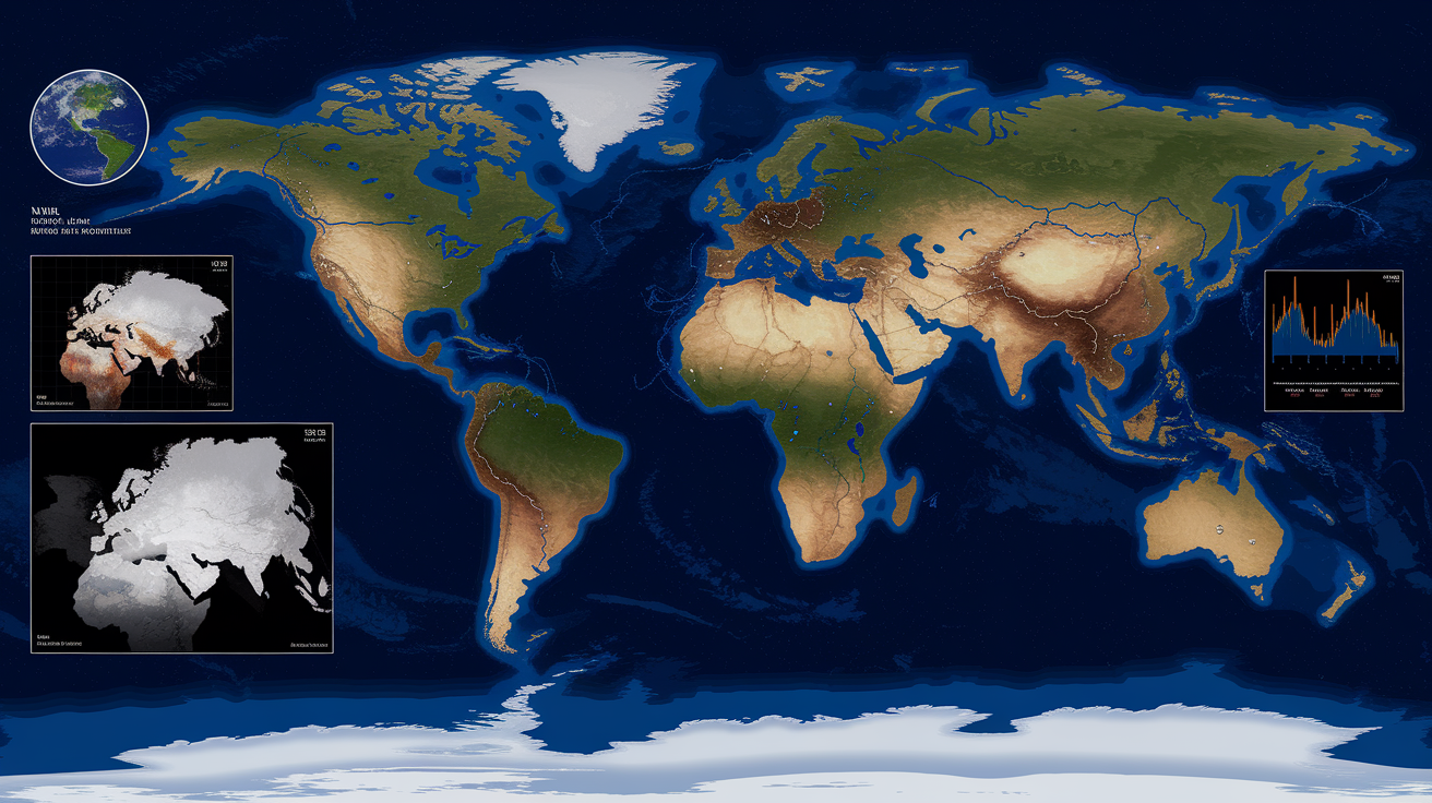
Satellite observations translate raw pixels into quantified environmental trends by combining imagery across time and applying algorithms that highlight change. Analysts calculate vegetation indices, dividing near-infrared reflectance by red reflectance to produce the Normalized Difference Vegetation Index, which rises when plants are healthy and falls during drought or deforestation. Change-detection methods compare images from different dates, flagging new buildings, floods, burned areas by identifying shifts in spectral signature. Digital Elevation Models derived from LiDAR or stereo radar pairs reveal topography, slope, drainage patterns essential for hydrology and landslide risk mapping. Cloud masking filters out pixels obscured by weather, ensuring only clear observations enter trend analyses.
These techniques have documented headline climate findings. Global surface temperature increased by 1.28 degrees Celsius compared to the 1880s baseline. Arctic sea ice extent declined at 12.2 percent per decade. Satellite records showed a 55 percent drop in Ganges River turbidity during COVID-19 lockdowns when industrial discharges paused. Time-series data also tracked a slight dip in India’s sulfur dioxide emissions between 2016 and 2019, mapped illegal logging in Arunachal Pradesh, revealed urban heat islands where built surfaces push local temperatures several degrees above vegetated areas.
Representative environmental metrics extracted from satellite imagery:
Arctic sea ice extent – Declining 12.2% per decade, measured via microwave radiometers that penetrate clouds.
Global mean temperature anomaly – +1.28°C above 1880s levels, derived from thermal infrared sensors and weather satellite networks.
Ganges turbidity change – 55% reduction during 2020 lockdown, quantified by comparing Sentinel-2 and Landsat-8 water-color bands.
Deforestation rate – Forest-cover loss in Western and Eastern Ghats tracked through annual NDVI and land-cover classifications.
Urban heat intensity – Surface temperature differences of 3–7°C between concrete and green spaces, mapped with thermal infrared data.
Real-World Applications of Earth Observation Systems
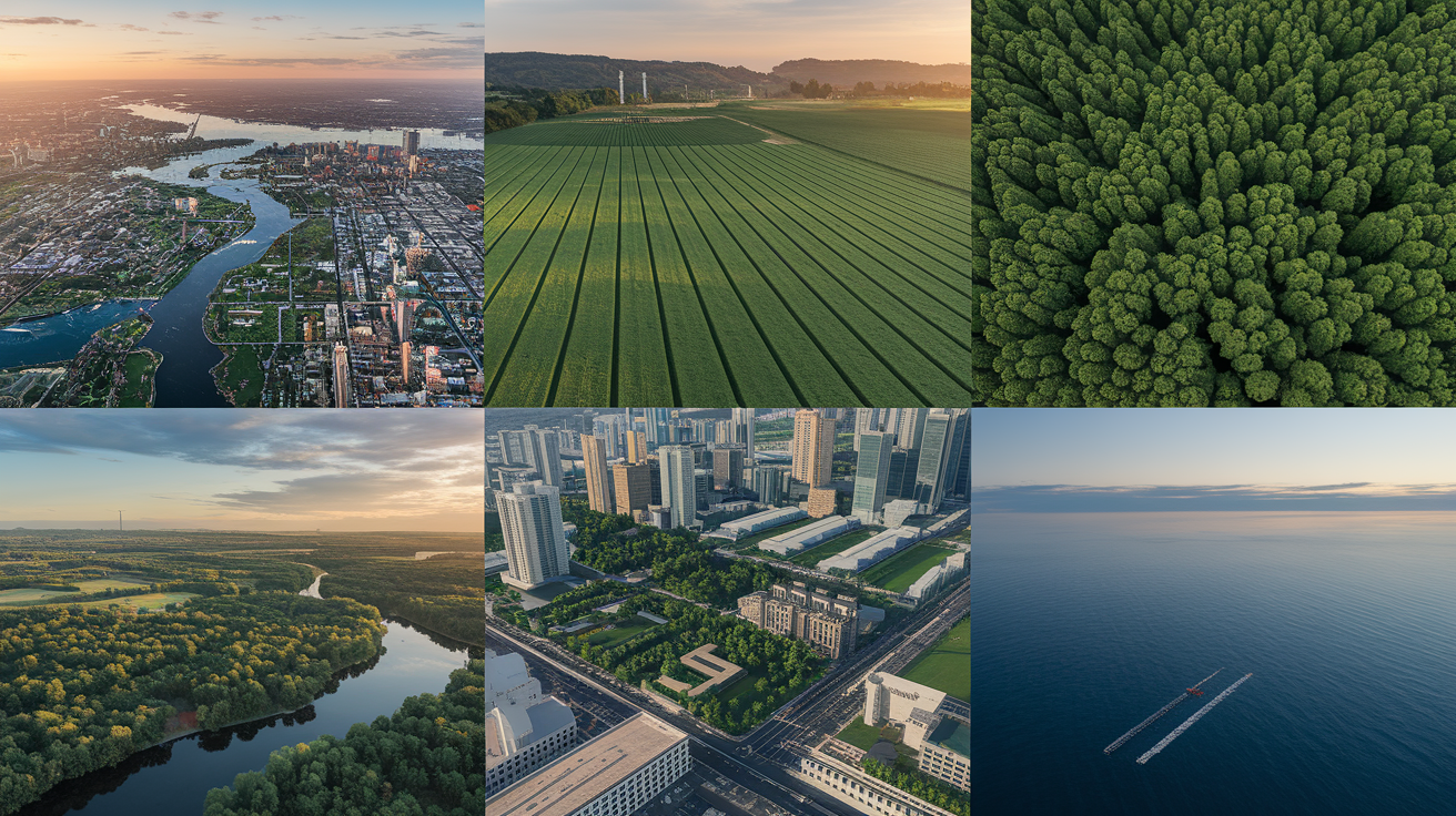
Earth observation satellites support decision-making across government, industry, research by delivering spatially explicit, repeatable measurements that ground surveys can’t match in speed or coverage. Disaster managers use wide-area flood maps generated within hours of heavy rain to direct evacuations and relief supplies. Wildfires are detected by thermal sensors that spot temperature spikes smaller than a pixel, triggering alerts before flames spread widely. Oil spills appear as dark slicks on SAR imagery because calm oil dampens wave roughness, enabling coast guards to track pollution and identify responsible vessels even at night or through fog.
Agriculture benefits from near-daily revisits that monitor crop emergence, growth stages, drought stress through NDVI time series, guiding precision irrigation and fertilizer application. Forestry agencies compare annual mosaics to quantify deforestation, illegal logging, habitat fragmentation. Satellite surveillance in Karnataka, for example, countered forest encroachment by providing evidence courts could verify. Urban planners overlay multispectral imagery with census data to map population density, infrastructure gaps, heat-island effects, informing green-space placement and zoning decisions. Coastal and marine observation tracks sea-surface temperature, algal blooms, fishing-zone productivity. India’s Oceansat and INSAT satellites feed data to fisheries managers who forecast potential catches and detect illegal trawling.
Climate researchers assemble decades of satellite records to measure glacier retreat, sea-level rise, greenhouse-gas proxies, building the long-term datasets that underpin international assessments. Air-quality agencies monitor nitrogen dioxide, sulfur dioxide, methane, particulate matter from space, identifying pollution hot spots and verifying emission-reduction policies like India’s National Clean Air Program. Health scientists are beginning to link satellite-derived environmental variables, standing water, vegetation density, temperature, to vector-borne disease risk, helping predict malaria and dengue outbreaks before they peak. Brief list of operational uses:
- Cyclone and storm tracking – Geostationary and polar satellites provide continuous wind, temperature, moisture profiles for early warnings.
- Flood extent mapping – Rapid SAR or optical imaging delineates inundated areas, supporting rescue and damage assessment.
- Wildfire detection and burn-scar mapping – Thermal sensors spot ignition. Follow-up imagery measures area burned and vegetation recovery.
- Deforestation monitoring – Annual or seasonal change detection flags illegal clearing and tracks reforestation efforts.
- Pollution tracking – Spectrometers measure NO₂, SO₂, methane columns. Time series reveal emission trends and compliance with air-quality standards.
- Fisheries zone forecasting – Sea-surface temperature and chlorophyll maps guide fleets to productive waters and reduce search time.
Spacecraft Engineering That Makes Observation Possible
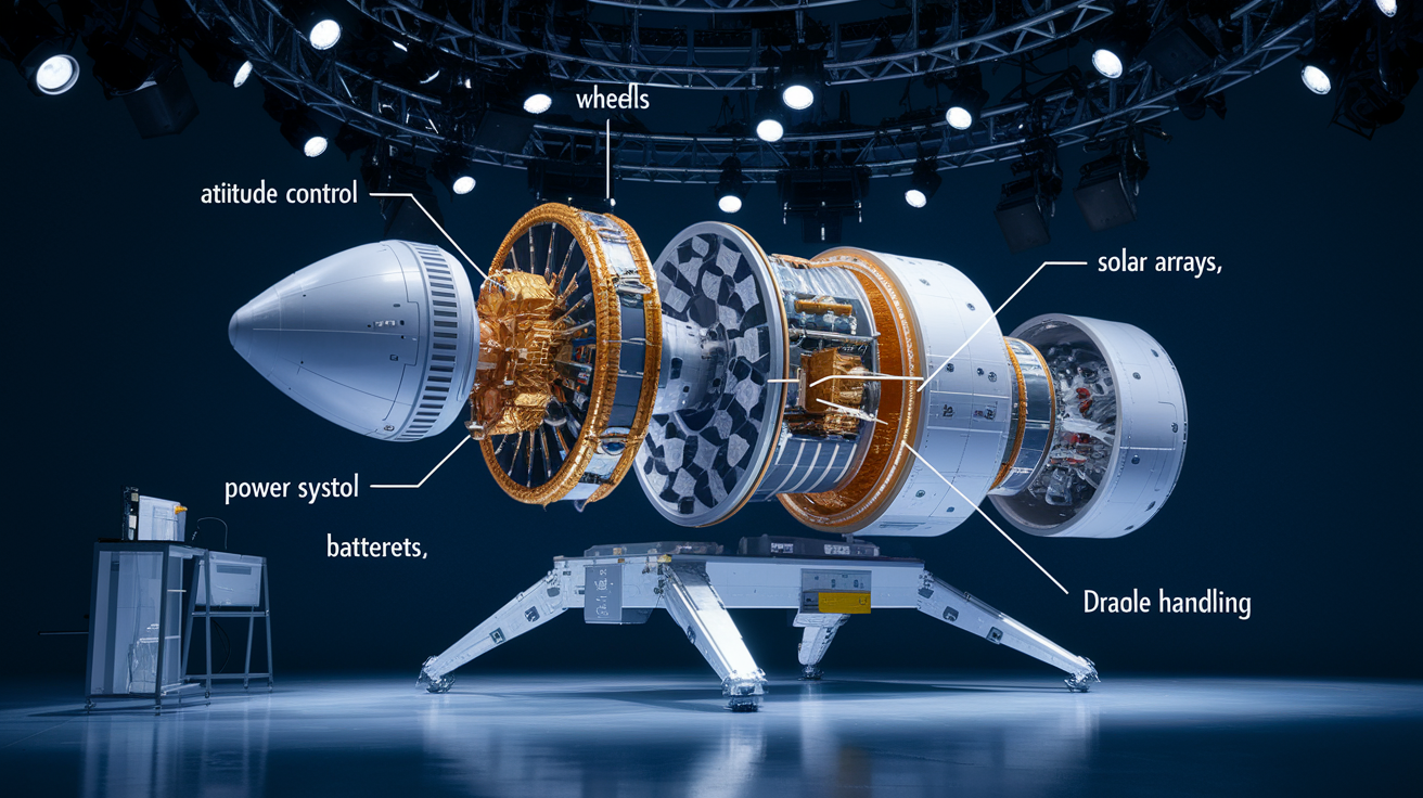
Behind every image lies a spacecraft bus, the structural platform and subsystems that keep sensors pointed, powered, thermally stable. Attitude control systems use reaction wheels, magnetic torquers, or thrusters to orient the satellite with sub-degree precision, ensuring each pixel falls on the intended ground location. Star trackers and gyroscopes measure orientation. Onboard computers send commands to actuators that correct drift caused by atmospheric drag or solar pressure. Pointing accuracy must hold steady during the seconds-long exposure required for high-resolution imaging. Vibrations from moving parts or thermal flexing are damped by isolation mounts and careful structural design.
Power systems rely on solar arrays that unfold after launch, tracking the Sun to harvest energy and charge lithium-ion batteries that sustain operations during eclipses. Battery management circuits balance charge across cells and prevent overheating, extending lifespan through thousands of charge-discharge cycles. Thermal control uses multi-layer insulation blankets, radiators, heaters to keep electronics within operating range, typically negative 10 to plus 50 degrees Celsius, despite wild swings between sunlit and shadowed passes. Onboard data storage employs solid-state recorders with tens to hundreds of gigabytes, buffering imagery until the next ground-station contact and prioritizing high-value scenes when memory fills. Payload integration mounts sensors on a stable optical bench, routes power and data buses, provides precise mechanical interfaces so that pointing knowledge translates into accurate geolocation. Key bus subsystems:
Attitude determination and control – Reaction wheels, star trackers, gyroscopes, control algorithms maintain precise pointing.
Power generation and storage – Solar arrays, batteries, power-conditioning electronics supply continuous energy.
Thermal management – Insulation, radiators, heaters regulate temperature across orbit day-night cycles.
Data handling – Solid-state recorders, onboard processors, downlink transmitters manage and deliver imagery.
Mission Lifecycles: Launch, Lifetime, and End-of-Life
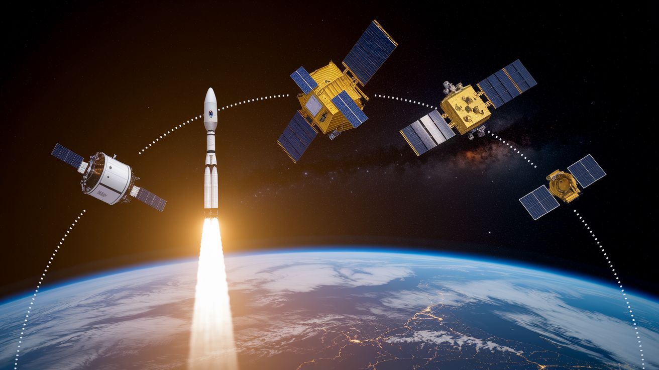
Earth observation missions begin with launch-vehicle selection based on satellite mass, target orbit, budget. Small satellites under 100 kilograms often ride as secondary payloads on rideshare missions, SpaceX Falcon 9 smallsat launches for example, cutting costs by sharing the ride with dozens of other spacecraft. Larger platforms require dedicated medium or heavy launchers that deliver them directly to sun-synchronous or geostationary transfer orbits. Once on orbit, mission operators commission the satellite by deploying solar panels, checking subsystems, calibrating sensors against known ground targets or stars. Operational lifetime typically spans 3 to 15 years, limited by fuel for attitude control, battery health, component radiation tolerance.
Standard end-of-life protocol calls for lowering the satellite to approximately 450 kilometers, where atmospheric drag pulls it down within one to two years, ensuring it burns up on re-entry and clears the crowded orbital environment. Recent research shows the thermosphere is shrinking due to greenhouse gases, reducing drag and extending decay times. Retired satellites may linger longer than planned, raising collision risk and complicating debris mitigation. Miniaturized constellations have changed the launch cadence. The first sub-100-kilogram SAR satellite launched in 2018, followed by 13 additional missions that built a fleet enabling daily revisits and persistent monitoring. Smallsats and CubeSats lower barriers to entry, letting universities, startups, developing nations deploy sensors that once required billion-dollar programs. Deorbit considerations:
Target altitude of ~450 km – Ensures natural re-entry within 1–2 years under historical drag estimates.
Thermosphere contraction – Shrinking atmosphere reduces drag, potentially doubling decay time and increasing debris risk.
Active removal – Future missions may use propulsion for controlled deorbit or on-orbit servicing to extend useful life and manage end-of-mission disposal responsibly.
Accessing Satellite Data and Tools for Using It
Open data programs have democratized access to Earth observation imagery. The European Union’s Copernicus initiative distributes Sentinel satellite data free of charge, covering optical, radar, atmospheric measurements with revisit times as short as five days. NASA and the U.S. Geological Survey maintain the Landsat archive, the longest continuous civilian Earth-imaging record, also available at no cost. Both programs deliver imagery in standard formats like GeoTIFF and NetCDF, readable by common geographic information system software and cloud platforms.
Cloud-based platforms host petabytes of satellite data and provide processing tools that run analyses without downloading raw files. Users search catalogs by location, date, sensor type. Apply atmospheric correction and index calculations on the fly. Export results as map layers or time-series charts. Application programming interfaces let developers automate data retrieval, trigger processing pipelines, integrate satellite insights into mobile apps or decision-support systems. Web viewers and visualization tools display multispectral composites, overlay change-detection results, animate time series, making complex datasets accessible to non-specialists. Steps to use satellite data:
Discover – Search open archives (Copernicus, Landsat) by location, date, cloud cover, sensor.
Process – Apply radiometric calibration, atmospheric correction, geometric alignment using cloud platforms or desktop GIS software.
Analyze – Calculate indices (NDVI, NDWI), classify land cover, detect changes, extract digital elevation models.
Visualize – Generate false-color composites, time-series animations, interactive web maps to communicate findings.
Final Words
We followed a satellite from orbit choice through sensors, data capture, downlink, and ground processing to the final maps analysts use.
We noted LEO vs GEO altitudes (~200–2,000 km vs 35,786 km), passive and active sensors (optical, thermal, SAR, LiDAR), and the core workflow: acquire, digitize, store, downlink, calibrate, analyze.
If you asked how do earth observation satellites work, they convert reflected or emitted energy into calibrated maps and measurements used for weather, climate, and disaster response. Better sensors and open data mean faster, clearer insights.
FAQ
Q: What do earth observation satellites do?
A: Earth observation satellites observe Earth’s surface, atmosphere and oceans, collecting imagery and measurements for weather, mapping, environmental monitoring, agriculture, disaster response and climate tracking using optical, thermal, radar and other sensors.
Q: Why don’t satellites fly over the poles?
A: Satellites don’t fly over the poles when they must stay fixed relative to Earth: geostationary satellites orbit above the equator at about 35,786 km, while polar or sun-synchronous satellites do pass over the poles for global coverage.
Q: Who owns most of the satellites?
A: Most satellites are owned by commercial operators today, with a few companies—especially SpaceX via Starlink—holding a large share; governments, defense agencies and scientific groups own the remaining satellites.
Q: Why is Elon Musk putting so many satellites in orbit?
A: Elon Musk is launching many satellites to build Starlink, a low‑Earth orbit broadband constellation that increases global internet coverage, reduces latency, and scales capacity to serve remote users and generate commercial revenue.