
Is hyperspectral always better than multispectral? Not really.
Multispectral satellites grab a few broad slices of color, while hyperspectral instruments record hundreds of narrow wavelength channels, giving a near-continuous spectrum (a light fingerprint) for every pixel.
That sounds technical, but it changes what you can see: crop stress, specific minerals, or just simple land cover.
This post breaks down the key differences, such as band count, spectral width, data size and common uses, so you can pick the right sensor for your problem.
Core Comparison: Multispectral vs Hyperspectral Satellite Differences Explained

Here’s the simplest way to think about it: multispectral satellites grab a few wide slices of the electromagnetic spectrum, while hyperspectral satellites measure hundreds of very narrow wavelength channels lined up side by side. Multispectral sensors usually capture somewhere between 3 and 10 bands. Sometimes it’s 4 to 12. Each one covers a pretty broad chunk of wavelengths—like a single band stretching from 640 to 670 nanometers for red light. Hyperspectral sensors work differently. They chop the spectrum into hundreds of narrow bands, often just 10 to 20 nanometers wide, stacking them to build what’s called a “hyperspectral cube.” Every pixel in that cube holds a near-continuous spectrum. It’s like taking a really fine-resolution light fingerprint of every single point on the ground.
Real numbers make this easier to picture. Landsat-8 is a widely used multispectral satellite. It collects 11 bands across visible, near-infrared, shortwave infrared, cirrus, and thermal wavelengths. Most bands sit at 30-meter spatial resolution. NASA’s Hyperion sensor launched in 2000 aboard the EO-1 satellite and it captures 242 hyperspectral bands spanning 0.4 to 2.5 micrometers. Still 30-meter resolution on the ground, but with way finer spectral slicing. That means Hyperion can spot tiny shifts in reflectance that Landsat’s broader bands would just smooth over. The catch? Hyperion’s data files are orders of magnitude larger and processing them takes more time, storage, and computing power.
Why hyperspectral forms a “cube” and multispectral doesn’t comes down to spectral sampling density. Multispectral data is discrete. A handful of separate band images stacked together like layers in a sandwich. Hyperspectral data gets sampled so densely that you can plot a full reflectance curve for each pixel, turning every image location into a continuous spectrum. That cube structure (spatial x-dimension, spatial y-dimension, and a spectral z-axis with hundreds of steps) unlocks new ways to analyze materials. But it also introduces redundancy between neighboring bands and demands sophisticated algorithms to keep processing manageable.
Key differences at a glance:
- Band count: multispectral 3–12 bands; hyperspectral hundreds (often 100–300+)
- Spectral width: multispectral bands tens to hundreds of nanometers wide; hyperspectral 10–20 nm
- Data structure: multispectral discrete layers; hyperspectral continuous per-pixel spectra (cube)
- File size and processing: hyperspectral tens to hundreds of times larger, requires dimensionality reduction and specialist software
- Spectral resolution: hyperspectral captures subtle material signatures invisible to multispectral sensors
Electromagnetic Spectrum Concepts for Understanding Spectral Satellites
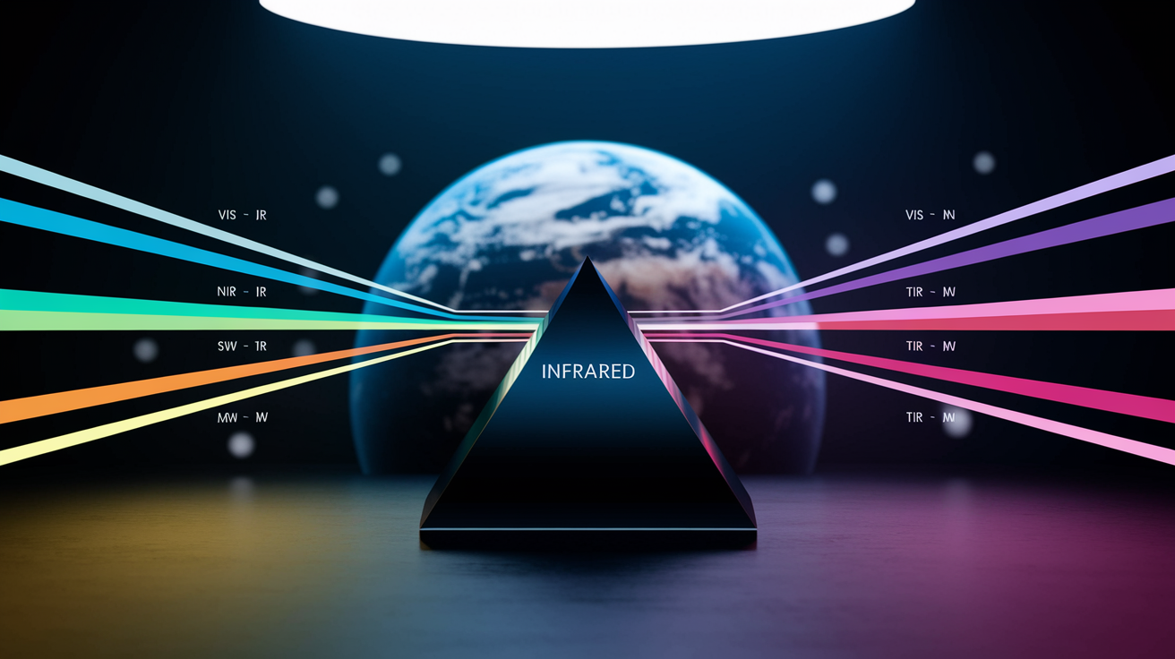
Understanding which parts of the electromagnetic spectrum satellites measure helps explain why sensors get designed the way they are. Visible light runs from about 400 to 700 nanometers. That’s the range human eyes see. Near-infrared sits just beyond that, roughly 700 to 1,000 nanometers, where healthy vegetation reflects strongly. Shortwave infrared extends from around 1,000 to 2,500 nanometers, revealing information about soil moisture, plant biochemistry, and mineral composition. Beyond that, thermal infrared and microwave regions exist. Most optical multispectral and hyperspectral satellites focus on the visible through shortwave infrared window because that’s where sunlight is strongest and materials show clear reflectance patterns.
There’s a practical gap worth noting. Earth’s atmosphere absorbs strongly between about 0.88 and 1.36 micrometers, making imaging in that slice difficult or impossible from space. Satellite sensor designers pick wavelength regions that avoid major absorption features and target specific applications. Coastal monitoring in the blue. Vegetation health in the red and near-infrared. Soil and minerals in the shortwave infrared. Multispectral sensors choose a few strategic bands in those useful zones. Hyperspectral sensors sample across the entire usable range with narrow, contiguous channels.
| Region | Wavelength Range | Common Uses |
|---|---|---|
| Visible (VIS) | 400–700 nm | True-color imaging, water clarity, basic land cover |
| Near-Infrared (NIR) | 700–1,000 nm | Vegetation health, biomass, leaf structure |
| Shortwave Infrared (SWIR) | 1,000–2,500 nm | Soil moisture, plant biochemistry, mineral identification |
| Thermal Infrared (TIR) | 8,000–14,000 nm | Surface temperature, fire detection, urban heat mapping |
| Microwave (MW) | 1 mm–1 m | Radar imaging, soil moisture, all-weather observation |
Multispectral Satellite Imaging Essentials

Multispectral systems split incoming light into a small number of wavelength channels. Each one’s carefully chosen to capture specific information about the ground. A typical multispectral satellite might have bands for coastal blue, standard blue, green, red, near-infrared, and one or two shortwave infrared channels. Enough to track vegetation health using indices like NDVI (Normalized Difference Vegetation Index), map water bodies, and classify broad land-cover types. Landsat-8 carries 11 bands, including coastal aerosol (0.43–0.45 micrometers), blue (0.45–0.51), green (0.53–0.59), red (0.64–0.67), NIR (0.85–0.88), two SWIR bands, a panchromatic band at 15-meter resolution, cirrus, and two thermal infrared bands at 100-meter resolution. Most optical bands sit at 30 meters per pixel, balancing coverage area with detail.
Sentinel-2 is part of the European Space Agency’s Copernicus program and provides free multispectral imagery at 10-meter resolution in its visible and NIR bands. Additional bands come at 20 and 60 meters covering red-edge, SWIR, and atmospheric correction wavelengths (ESA Copernicus Sentinel data). Commercial satellites like WorldView-2, -3, and -4 push spatial resolution below 0.5 meters while still capturing multiple spectral bands. That enables detailed mapping of urban infrastructure, crop rows, and small-scale environmental features. These multispectral platforms revisit the same location frequently. Sentinel-2’s two-satellite constellation offers a five-day global revisit, making them ideal for monitoring changes over time.
Why multispectral systems dominate operational remote sensing comes down to practical advantages:
- High spatial resolution: Commercial multispectral satellites can resolve features smaller than half a meter, far sharper than most hyperspectral systems.
- Smaller data volumes: Fewer bands mean smaller file sizes, faster downloads, and lower storage costs. Important when covering large areas repeatedly.
- Fast processing workflows: Standard software packages and well-established algorithms (NDVI, land-cover classification, change detection) make multispectral data quick to analyze.
- Widely available free imagery: Landsat and Sentinel-2 archives stretch back decades and cover the entire planet, with no cost for access and redistribution.
Hyperspectral Satellite Imaging Essentials

Hyperspectral sensors flip the logic. Instead of picking a handful of strategic bands, they measure reflectance across hundreds of narrow, contiguous wavelength channels, building a complete spectrum for every pixel. NASA’s Hyperion sensor was one of the first successful spaceborne hyperspectral imagers. It captured 242 bands from 0.4 to 2.5 micrometers at 30-meter spatial resolution after its launch in 2000. Each band was about 10 nanometers wide. Narrow enough to detect subtle absorption features tied to specific minerals, plant pigments, or chemical compounds. Later missions (PRISMA from Italy in 2019, EnMAP from Germany in 2020, HISUI from Japan in 2020) have continued refining hyperspectral capabilities, improving signal-to-noise ratios, onboard calibration, and data delivery speeds.
The power of hyperspectral imaging lies in its ability to identify materials by their spectral fingerprints. Mining geologists can distinguish between three visually similar minerals because each absorbs light differently at precise wavelengths in the shortwave infrared. Agricultural researchers can detect early vegetation stress by tracking shifts in the red-edge region. That’s the steep slope between red and near-infrared reflectance, where even small changes in chlorophyll concentration alter the curve shape. Water-quality specialists can measure specific algal pigments or dissolved organic matter by isolating narrow absorption bands that multispectral sensors would lump together with neighboring wavelengths.
The downside: hyperspectral data volumes are huge. A single Hyperion scene with 242 bands contains roughly 20 times more information than a comparable Landsat scene with 11 bands. That ratio grows with newer sensors pushing past 300 bands. Storage, bandwidth, and processing all scale up. Atmospheric correction becomes more critical because narrow bands amplify the impact of scattering and absorption by gases and aerosols. And there’s redundancy. Adjacent hyperspectral bands often look very similar, which is why analysts use dimensionality-reduction techniques like Principal Component Analysis or Minimum Noise Fraction to compress the data before classification.
Continuous Narrowband Sampling
What makes hyperspectral unique is the near-continuous spectral curve you get for each pixel. Picture a reflectance graph with wavelength on the x-axis and reflectance percentage on the y-axis. A multispectral sensor gives you a handful of dots on that graph, one per band. A hyperspectral sensor gives you hundreds of closely spaced dots. Enough to draw a smooth curve showing every dip and peak caused by molecular absorption and scattering. That curve is the material’s spectral signature, and it’s detailed enough to identify not just “vegetation” but specific plant species. Not just “rock” but the exact mineral assemblage.
This resolution matters when targets look similar in broad bands but differ in narrow features. Three minerals might all reflect about 30 percent of light in a wide SWIR band centered at 2,200 nanometers. But zoom in with 10-nanometer hyperspectral channels and you’ll see one mineral has an absorption dip at 2,160 nm, another at 2,200 nm, and the third at 2,240 nm. A multispectral sensor averaging across that range would miss the distinction entirely. Hyperspectral imaging picks it up, enabling precise mineral mapping critical for exploration and environmental monitoring.
The same principle applies to vegetation. Healthy leaves, water-stressed leaves, and leaves with early disease might all show high NIR reflectance in a broad multispectral band. But hyperspectral sensors can measure the exact position and depth of the red-edge slope. They detect subtle shifts in chlorophyll absorption around 680 nm. They identify changes in leaf water content via fine absorption features near 1,450 nm and 1,950 nm. That granularity turns “green stuff” into actionable information about crop health, invasive species presence, or ecosystem stress before visible symptoms appear.
Technical Differences in Spectral Resolution, Data Volume, and Processing Workflows
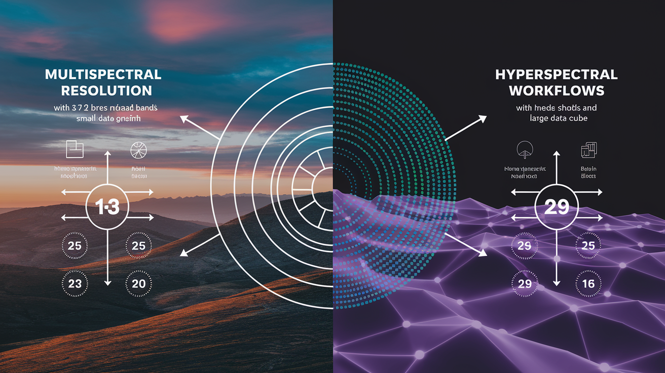
Spectral resolution defines how finely a sensor divides the electromagnetic spectrum. Multispectral sensors have low spectral resolution. Each band covers a relatively wide wavelength slice. But they compensate with high spatial resolution, frequent revisits, and manageable data sizes. Hyperspectral sensors have high spectral resolution, slicing the spectrum into narrow channels that reveal fine material signatures. That precision comes at the cost of larger data files, lower spatial sharpness in many systems, and longer processing pipelines. The trade isn’t arbitrary. Sensor designers balance the number of photons entering each detector against the noise floor. Narrower spectral bands mean fewer photons per channel, which can reduce image quality unless exposure times or sensor sensitivity increase.
Data volume differences are stark. A single Landsat-8 scene covering about 185 by 180 kilometers with 11 bands and 30-meter pixels produces roughly 1 gigabyte of data. A hyperspectral sensor imaging the same area with 200 bands at the same spatial resolution generates 20 gigabytes or more, depending on bit depth. Modern hyperspectral missions often use 12- or 16-bit encoding per pixel to preserve radiometric fidelity. Many multispectral systems stick with 8- or 11-bit. Higher bit depth multiplies file sizes again. When you’re covering large regions or building time-series datasets, those numbers add up fast, driving storage costs and complicating data distribution.
Processing workflows diverge just as sharply. Multispectral data typically follows a straightforward path: radiometric calibration converts raw digital numbers to at-sensor radiance, atmospheric correction removes scattering and absorption effects to produce surface reflectance, and then analysts calculate vegetation indices, run supervised classifications, or apply change-detection algorithms using standard software packages. Total processing time for a multispectral scene might be minutes to a few hours on a modern workstation. Hyperspectral workflows require all those steps plus dimensionality reduction (PCA, MNF, or targeted band selection) to manage redundancy. Spectral unmixing to separate mixed pixel signatures. Often custom algorithm development because off-the-shelf tools don’t always handle hundreds of bands efficiently. Processing a hyperspectral scene can take days, especially when atmospheric correction demands per-band tuning and validation.
Onboard satellite constraints also matter. Telemetry bandwidth limits how much data a satellite can downlink during each ground-station pass. A hyperspectral sensor generating tens of gigabytes per orbit either needs onboard compression (which can introduce artifacts), selective imaging (capturing only high-priority targets), or larger downlink antennas and higher transmission rates. Some missions solve this by delivering only a subset of bands in near-real-time, with the full hyperspectral cube available later after reprocessing on the ground. Multispectral satellites face fewer bottlenecks, enabling more frequent imaging and faster delivery to users.
| Attribute | Multispectral | Hyperspectral |
|---|---|---|
| Number of Bands | 3–12 (typically 4–10) | Hundreds (100–300+) |
| Spectral Width per Band | Tens to hundreds of nanometers | 10–20 nanometers |
| Data Volume (relative) | Baseline (e.g., 1 GB per scene) | 20–100× larger |
| Processing Complexity | Standard corrections and indices | Dimensionality reduction, unmixing, specialist algorithms |
| Typical Spatial Resolution | 0.5–30 m (often higher) | 15–30 m (sometimes coarser) |
| Common Software | QGIS, ArcGIS, ENVI, Google Earth Engine | ENVI, SpecTIR, custom Python/R pipelines |
Sensor Platforms and Real-World Satellite Examples
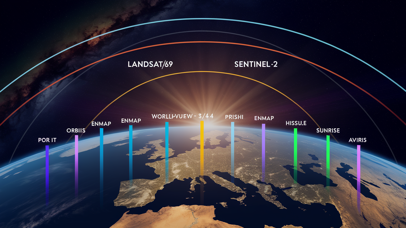
Multispectral and hyperspectral sensors fly on a mix of government, commercial, and research satellites. Each gets optimized for different mission goals. Landsat-8 and Landsat-9 are operated by NASA and the U.S. Geological Survey. They provide free, global multispectral coverage every 16 days at 30-meter resolution, with a data archive stretching back to 1972 across the Landsat series. Sentinel-2A and -2B are part of Europe’s Copernicus program. They offer 10-meter visible and NIR bands with a combined five-day revisit. Also free and open. Commercial multispectral providers like Maxar’s WorldView constellation deliver sub-meter imagery. WorldView-3 reaches 0.31-meter panchromatic and 1.24-meter multispectral resolution. Higher cost but with tasking flexibility and rapid revisit over high-priority areas.
On the hyperspectral side, Hyperion aboard NASA’s EO-1 satellite pioneered spaceborne hyperspectral imaging from 2000 to 2017. It proved the technology but revealed the challenges of data volume and atmospheric correction. Italy’s PRISMA (launched 2019) and Germany’s EnMAP (2020) represent the current generation, offering 30-meter hyperspectral cubes with improved calibration, onboard processing, and faster ground delivery. Japan’s HISUI hyperspectral sensor got installed on the International Space Station in 2020. It tests even more advanced detectors and onboard compression. NASA has proposed future missions like HyspIRI (planned around 2024, though timelines shift) to push hyperspectral capabilities further, potentially combining thermal and reflected-light hyperspectral imaging on a single platform.
Airborne systems like NASA’s AVIRIS (Airborne Visible/Infrared Imaging Spectrometer) fill a different niche. AVIRIS captures 224 contiguous hyperspectral bands from aircraft, achieving spatial resolutions as fine as a few meters depending on flight altitude. Because airborne platforms fly lower and slower than satellites, they can image smaller areas with higher detail and more flexible scheduling. That makes them ideal for research campaigns, disaster response, and detailed site surveys. The trade: airborne coverage is limited compared to satellites, and costs per square kilometer are higher. Many projects use satellite multispectral data for broad monitoring and airborne hyperspectral for targeted follow-up.
Typical platform capabilities:
- Landsat-8/9: 11 multispectral bands, 30 m spatial resolution (15 m pan, 100 m thermal), 16-day revisit, free global archive
- Sentinel-2: 13 multispectral bands, 10–60 m resolution, 5-day combined revisit, free access
- WorldView-3: 8 multispectral VNIR bands, 8 SWIR bands, 1.24 m multispectral resolution, tasking on demand
- PRISMA: ~240 hyperspectral bands (0.4–2.5 µm), 30 m resolution, tasking requests, calibrated data products
- AVIRIS (airborne): 224 hyperspectral bands, <5 m resolution achievable, flexible campaign scheduling
Applications Comparing Multispectral and Hyperspectral Capabilities
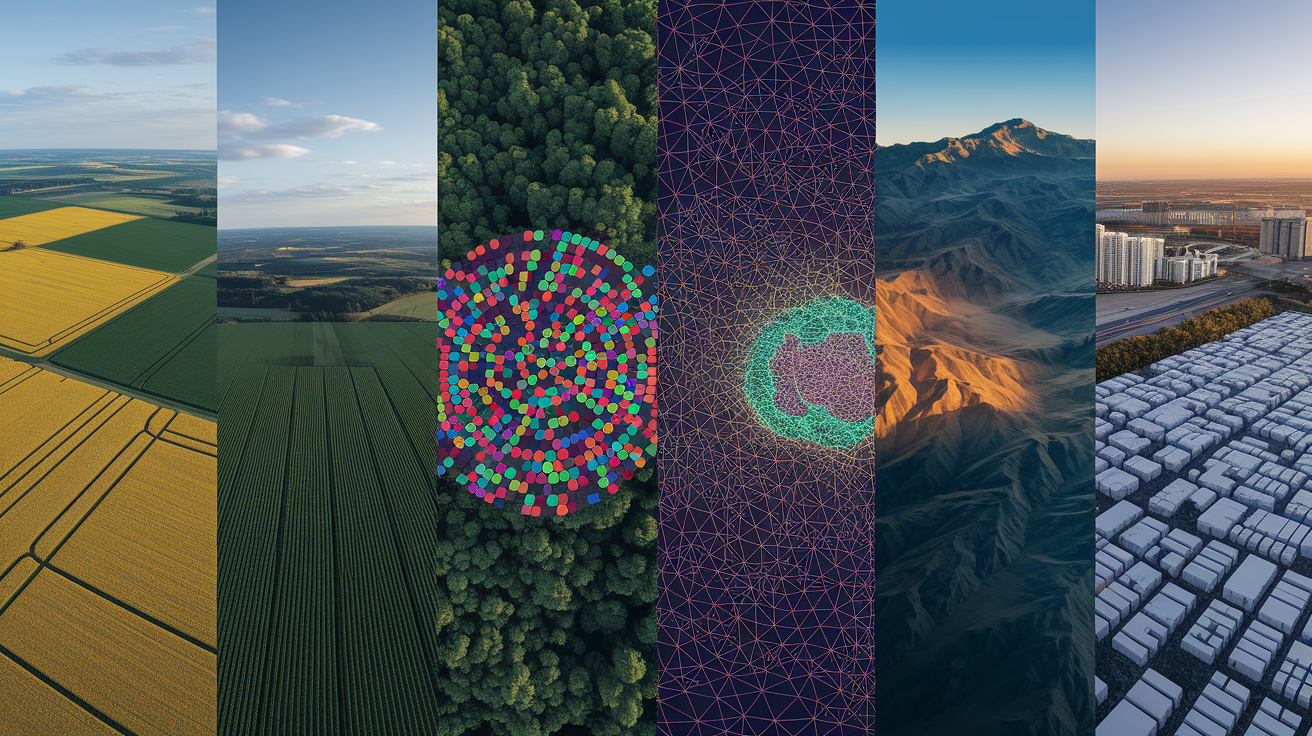
The choice between multispectral and hyperspectral often hinges on what you need to distinguish and how much detail matters. Multispectral sensors excel at broad classification tasks: mapping cropland versus forest, identifying water bodies, tracking urban expansion, and monitoring vegetation health using established indices like NDVI (Normalized Difference Vegetation Index) or EVI (Enhanced Vegetation Index). These indices combine reflectance from a red band and a near-infrared band to estimate chlorophyll content and biomass. They work well when the goal is to spot general health trends across large areas. Landsat-8 has been used to detect algal blooms in lakes by measuring increased green reflectance and reduced NIR penetration in water. A straightforward two-band signal that doesn’t require hyperspectral precision.
Hyperspectral sensors shine when targets are spectrally similar in broad bands but differ in narrow features. Separating three closely related tree species in a mixed forest might be impossible with Landsat’s six optical bands. They all look green and reflect NIR strongly. But hyperspectral data capturing the red-edge slope and subtle chlorophyll absorption differences can distinguish them, enabling species-level forest inventories. A 2020 study used multispectral Landsat time series to track changes in tree-species distribution. It noted that visible-only assessment missed critical information locked in NIR and red-edge wavelengths, information that hyperspectral sensors would capture directly. In mineral exploration, hyperspectral imaging identifies specific minerals (calcite, dolomite, kaolinite) by their unique absorption features in the SWIR. A task far beyond multispectral Thematic Mapper bands, which simply can’t resolve the narrow dips that define each mineral.
Precision agriculture sits somewhere in the middle. Multispectral drones and satellites provide cost-effective NDVI maps that guide variable-rate fertilizer application and irrigation scheduling across entire farms. Hyperspectral systems add value when farmers need early disease detection. Fungal infections or nutrient deficiencies often alter leaf biochemistry before visible symptoms appear, and those changes show up as shifts in narrow absorption bands around 550 nm (carotenoids) or 680 nm (chlorophyll). Water-quality monitoring follows a similar pattern: multispectral sensors flag general turbidity and algae presence; hyperspectral sensors quantify concentrations of specific pigments like chlorophyll-a or phycocyanin, enabling more precise bloom predictions and pollution source tracking.
Disaster response and rapid mapping lean heavily on multispectral systems because speed and coverage matter more than spectral detail. After a flood, wildfire, or earthquake, emergency managers need updated imagery within hours to assess damage extent and route aid. Multispectral satellites with daily or better revisit and fast processing pipelines deliver that. Hyperspectral data might arrive days later, after the immediate crisis has passed, though it can support follow-on environmental assessments. Mapping fire burn severity via mineral alteration signatures or tracking post-flood sediment chemistry.
Sector-by-Sector Comparison
-
Agriculture: Multispectral NDVI and crop health indices are standard for field-scale monitoring; hyperspectral detects early disease, nutrient stress, and species-level weed identification when precision justifies the cost.
-
Water quality: Multispectral identifies algal blooms and general turbidity (Landsat-8 example); hyperspectral quantifies specific pigment concentrations and dissolved organic compounds for regulatory reporting and research.
-
Mineral exploration: Multispectral can map broad alteration zones (iron oxides, clays); hyperspectral distinguishes individual mineral species critical for ore-deposit modeling. Over 4,000 mineral types exist, each with unique spectral composition.
-
Vegetation and forestry: Multispectral classifies land cover and estimates biomass via indices; hyperspectral enables species-level mapping, invasive-species detection, and biochemical parameter estimation (leaf area index, canopy nitrogen).
-
Urban and infrastructure mapping: Multispectral high-resolution imagery (WorldView) maps buildings, roads, and land use efficiently; hyperspectral adds material identification (asphalt type, roofing materials) for specialized engineering or environmental studies.
-
Disaster response: Multispectral dominates due to fast revisit, wide coverage, and rapid processing; hyperspectral supports post-event environmental impact assessments when detailed material or chemical mapping is needed.
Practical Guidelines: Choosing Between Multispectral and Hyperspectral Satellites

Start by defining your objective in concrete terms. What are you trying to detect, measure, or classify, and how much spectral detail does that require? If the answer is “track vegetation health across a region” or “map water extent after a storm,” multispectral is almost always the right tool. It’s faster, cheaper, and the data pipelines are well established. If the answer is “identify which mineral is exposed in this outcrop” or “detect early blight in tomato plants before visible symptoms,” hyperspectral becomes necessary because the spectral signatures you need are narrow and easily missed by broad bands. The core question: do you need to see subtle, material-specific absorption features, or will a handful of strategic wavelength windows suffice?
Budget and infrastructure matter just as much as the science. Hyperspectral systems cost more at every stage: sensor tasking fees are higher, data storage scales up by factors of 20 to 100, processing requires specialist software and more computing power, and interpretation often demands domain expertise (spectroscopy, mineralogy, plant physiology) that general remote-sensing staff may lack. Multispectral data, especially from free sources like Landsat and Sentinel-2, keeps costs low and fits into existing GIS workflows with minimal training. If your project has limited funding, tight timelines, or relies on regular updates (weekly or monthly monitoring), multispectral is the pragmatic choice. Hyperspectral makes sense when the added spectral information delivers measurable value. Better ore targeting, earlier crop intervention, regulatory compliance for water chemistry. Things that justify the investment.
Decision checklist for sensor selection:
- Spectral granularity needed: Can your target be identified with 4–12 broad bands, or do you need hundreds of narrow channels to resolve specific absorption features?
- Spatial resolution requirement: Do you need sub-meter detail (favoring multispectral), or is 15–30 m acceptable if spectral detail is high (hyperspectral)?
- Temporal frequency: Is frequent revisit critical (multispectral advantage), or is occasional targeted imaging sufficient (hyperspectral)?
- Data volume and processing capacity: Can your team handle tens of gigabytes per scene and run dimensionality-reduction algorithms, or do you need streamlined, fast-turnaround workflows?
- Budget for acquisition, storage, and software: Are funds available for hyperspectral tasking fees, expanded storage infrastructure, and specialist software licenses?
- Downstream analysis tools: Does your existing software stack support hyperspectral formats and algorithms, or would you need to build custom pipelines?
- Expertise availability: Do you have staff trained in spectroscopy and advanced remote sensing, or will you rely on simpler, index-based analysis methods?
Future Trends in Multispectral and Hyperspectral Satellite Technology
The line between multispectral and hyperspectral is starting to blur as sensor technology improves. New satellite designs pack more spectral bands into smaller, lighter instruments. Commercial providers are launching “superspectral” sensors with 20 to 50 bands. More than traditional multispectral but fewer than full hyperspectral, targeting sweet spots for specific industries. Miniaturization is a big driver. Hyperspectral sensors that once required large, expensive satellites can now fit on cubesats. That lowers launch costs and enables constellations of hyperspectral imagers that improve revisit rates. Onboard processing and compression algorithms are getting smarter, reducing the data bottleneck by transmitting only the most informative bands or running initial classifications in orbit before downlinking results.
Data fusion is another major trend. Combining multispectral imagery’s high spatial resolution and frequent revisit with hyperspectral’s spectral detail creates hybrid products that use the strengths of both. Machine-learning models trained on hyperspectral reference libraries can be applied to multispectral time series, effectively “upsampling” spectral information where hyperspectral coverage is sparse. Cloud-based processing platforms are making hyperspectral data more accessible, handling the storage and computation challenges that once limited hyperspectral analysis to specialized labs. As these platforms mature, the cost and expertise barriers will drop, and hyperspectral workflows will become routine for more users.
Key innovations on the horizon:
- Miniaturized hyperspectral sensors on cubesats: Smaller, cheaper satellites enabling hyperspectral constellations with improved temporal coverage
- Onboard AI and compression: Satellites running edge-computing algorithms to reduce downlink volume and speed delivery of actionable products
- Superspectral sensors (20–50 bands): Bridging multispectral and hyperspectral for targeted applications without full hyperspectral overhead
- Cloud-native analysis platforms: Centralized processing and storage reducing the infrastructure burden for end users and democratizing access to hyperspectral data
Final Words
In the action, we ran through the core differences: multispectral uses a few broad bands (Landsat: 11) while hyperspectral captures hundreds of narrow bands (Hyperion: 242).
We explained the spectral cube idea, gave sensor examples, and laid out data, processing, and application tradeoffs for vegetation, minerals, water, and mapping.
That brings us to the practical bottom line — how multispectral and hyperspectral satellites differ: choose multispectral for frequent, smaller-data monitoring and hyperspectral when you need fine spectral fingerprints. Both are useful, depending on the question.
FAQ
Q: What is the fundamental difference between multispectral and hyperspectral satellites?
A: The fundamental difference between multispectral and hyperspectral satellites is band detail: multispectral uses a few broad bands, while hyperspectral captures hundreds of narrow, contiguous bands for much finer spectral detail.
Q: How many spectral bands do multispectral and hyperspectral sensors typically have?
A: The number of spectral bands is: multispectral usually 3–10 (commonly 4–12); hyperspectral typically around 100–300+ bands, for example Landsat‑8 has 11 bands and Hyperion had 242 bands.
Q: Why is hyperspectral data described as a “cube” and multispectral as discrete stacks?
A: Hyperspectral data is a cube because it adds a continuous spectral axis to x,y images, forming a 3D block. Multispectral is discrete band stacking with separate, wider slices of that spectral axis.
Q: How do spectral resolution and band width differ between the two systems?
A: Spectral resolution differs by band width: hyperspectral bands are narrow (often ~10–20 nm), giving fine spectral resolution. Multispectral bands are much broader, reducing the ability to separate similar materials.
Q: What typical spatial resolutions do multispectral and hyperspectral satellites offer?
A: Typical spatial resolutions: multispectral ranges from <0.5 m (WorldView) to 10–30 m (Sentinel‑2, Landsat‑8). Hyperspectral satellites like Hyperion often sit near 30 m, though airborne systems can be much finer.
Q: What are the main application differences between multispectral and hyperspectral imaging?
A: Main application differences are: multispectral suits NDVI, land cover, and rapid monitoring. Hyperspectral excels at mineral ID, species discrimination, and detecting subtle biochemical changes in vegetation or water.
Q: How do data volume and processing needs compare between multispectral and hyperspectral?
A: Data volume and processing: hyperspectral generates orders of magnitude more data, requiring radiometric and atmospheric correction, dimensionality reduction (PCA/MNF), and unmixing. Multispectral needs less storage and faster workflows.
Q: When should I choose multispectral versus hyperspectral for a project?
A: You should choose multispectral for frequent, cost‑effective monitoring and quick analysis. Choose hyperspectral when you need fine spectral detail for species, mineral, or biochemical detection despite higher cost and processing needs.
Q: What are real satellite and sensor examples of each type?
A: Real examples: multispectral — Landsat‑8 (11 bands), Sentinel‑2 (10 m free imagery), WorldView (<0.5 m commercial). Hyperspectral — Hyperion (242 bands), PRISMA, EnMAP, HISUI, plus airborne AVIRIS systems.
Q: What future trends are emerging in multispectral and hyperspectral satellite technology?
A: Future trends include miniaturized hyperspectral sensors, better onboard compression and processing, more data fusion across sensors, and upcoming missions like HyspIRI improving access and capabilities.