
What if a satellite could read a rock like a barcode?
It can.
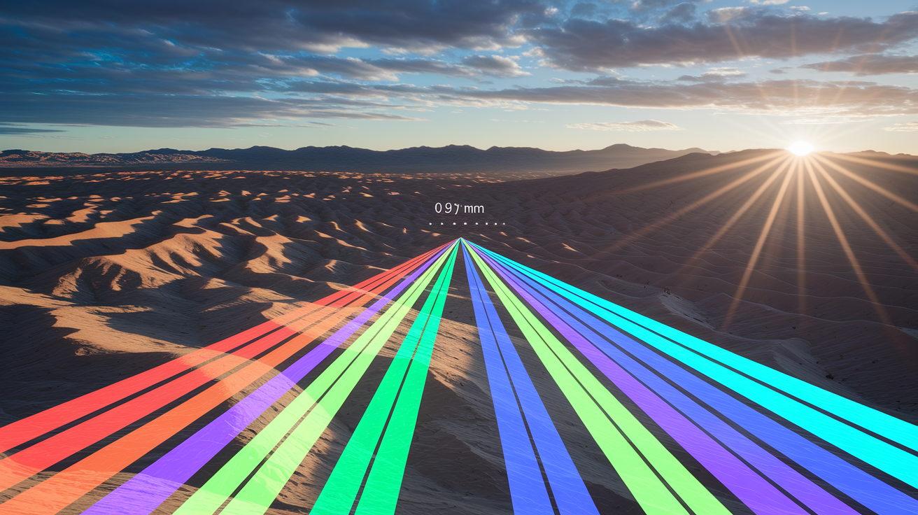
Sunlight hits a mineral, some wavelengths get absorbed and others bounce back.
Orbital sensors catch that returned light and turn it into a reflectance curve — the mineral’s fingerprint.
By analyzing those absorption troughs and their positions, scientists can tell clays from carbonates or hematite from goethite without leaving the plane.
This post explains how wavelength analysis does the work, what sensors need, and why remote mineral ID speeds exploration and mapping.
How Orbital Sensors Use Spectral Signatures to Identify Minerals
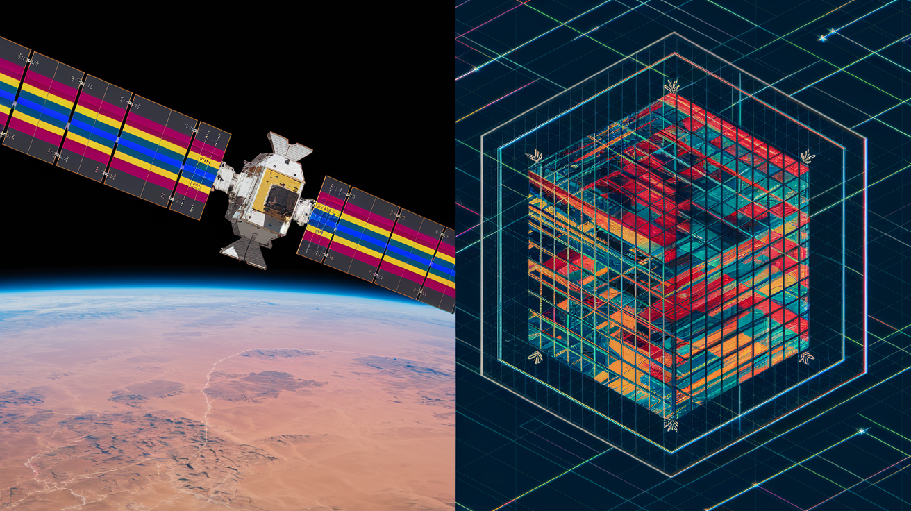
Orbital sensors spot minerals by measuring reflected sunlight across hundreds of narrow wavelength slices. Sunlight hits a mineral, certain wavelengths get absorbed, and others bounce back toward the satellite. The sensor catches that returning light as radiance, then converts it to reflectance by comparing it to the incoming solar energy. That reflectance curve is the mineral’s fingerprint.
Minerals absorb energy at particular wavelengths because of how their atoms vibrate or electrons jump between levels. Iron minerals pull energy out near 0.9 micrometers (µm) through electronic transitions. Clay minerals with hydroxyl groups (OH) absorb hard around 1.4 µm and 2.2 µm because those bonds resonate there. Carbonates show dips around 2.3 µm tied to CO₃ vibrations. Each mineral class stamps a distinct pattern of absorption troughs across the spectrum, and orbital sensors are designed to capture enough detail to separate one mineral from another.
The sensor’s task is converting raw radiance into calibrated reflectance spectra that can be matched against known mineral patterns. Onboard calibration targets track drift. Atmospheric correction strips out absorptions from gases and aerosols between the ground and the satellite. What’s left is ground reflectance ready for library comparison. Better spectral resolution (narrower bands) and higher signal to noise mean the sensor can resolve subtle features and tell similar minerals apart.
The standard detection workflow goes like this:
Radiance acquisition: The sensor records at sensor radiance across its full range, usually visible through shortwave infrared (VNIR to SWIR, roughly 0.4 to 2.5 µm).
Radiometric calibration: Raw counts become calibrated radiance using onboard references and pre flight data.
Atmospheric correction: A radiative transfer model or empirical method removes atmospheric effects to produce surface reflectance.
Spectral feature extraction: Algorithms locate absorption band centers, depths, and shapes by comparing reflectance to a smooth background curve.
Library matching: Extracted features get compared to reference spectra, and similarity scores assign the best mineral match to each pixel.
Fundamentals of Spectral Signatures in Mineralogy

A spectral signature is the reflectance curve you get when electromagnetic radiation interacts with a mineral’s crystal lattice and chemical bonds. Photons hit the surface. Some scatter, some penetrate and get absorbed by electronic or vibrational processes, the rest reflect. Which wavelengths disappear depends on composition and structure. Iron in oxidized form (Fe³⁺) absorbs visible and near infrared light differently than reduced iron (Fe²⁺), so hematite and magnetite have different curves even though both are iron oxides.
Absorption features appear as downward dips in reflectance. These dips tie to physical mechanisms. Electronic transitions, where electrons jump between energy levels in metals like iron or chromium, dominate the visible and near infrared. Vibrational modes, where molecular bonds stretch or bend at specific frequencies, control absorptions in the shortwave and thermal infrared. Hydroxyl bonds (O–H) vibrate near 1.4 µm and 2.2 µm, so any mineral with water or OH groups shows troughs there. Clays, micas, amphiboles. Carbonate minerals absorb near 2.3 µm because of the asymmetric stretch of the CO₃ ion.
Position, depth, and width of these bands encode mineral identity, composition, sometimes structure. A shift of a few tens of nanometers in a clay absorption from 2.20 µm to 2.21 µm can signal a change from montmorillonite to kaolinite. That kind of detail needs high spectral resolution and tight calibration, which is why hyperspectral sensors with narrow, contiguous bands are the tool for orbital mineral mapping.
Orbital Sensor Types and Their Relevance to Mineral Mapping
Orbital sensors split into two camps: multispectral and hyperspectral. Multispectral sensors grab data in a handful of wide bands, typically 4 to 15, spread across visible, near infrared, sometimes shortwave infrared. Sensors like Landsat OLI or Sentinel-2 MSI work well for broad land cover and can separate major mineral groups (iron oxides versus clays, for instance) using band ratios. They can’t resolve the narrow features you need to pin down specific minerals within a group.
Hyperspectral sensors collect hundreds of contiguous narrow bands, often with spectral sampling around 5 to 10 nanometers. This fine sampling grabs the full shape of absorption features, so you can tell kaolinite from montmorillonite or goethite from hematite. Hyperion flew on NASA’s EO-1 from 2000 to 2017 and delivered around 220 bands from 0.4 to 2.5 µm. PRISMA, launched by the Italian Space Agency in 2019, offers more than 230 bands over the same range. EnMAP, a German mission from 2022, pushes roughly 240 bands with better signal to noise in the SWIR. Airborne platforms like AVIRIS-NG give even finer spatial resolution (sub meter to a few meters) and can target specific sites.
Sensor performance for mineral mapping depends on three resolutions. Spectral resolution is band width and spacing. Narrower is better for diagnostic features. Spatial resolution is ground sampling distance (GSD). Finer pixels cut down on mixing different materials within a pixel, which helps detectability. Radiometric resolution is how well the sensor distinguishes small radiance differences. Higher bit depth and careful calibration boost signal to noise, critical when absorption features are shallow or the target mineral covers just part of the pixel.
Key Wavelength Regions for Mineral Detection

Mineral detection from orbit leans on three wavelength zones, each tied to different physics. Visible to near infrared (VNIR, roughly 0.4 to 1.0 µm) captures electronic absorptions in iron bearing minerals and surface color. Iron oxides like hematite and goethite show strong absorptions near 0.5 to 0.9 µm, and the exact position and shape help separate oxidation states and phases. VNIR is also sensitive to vegetation and organic coatings, which can hide mineral signals if you’re not careful.
Shortwave infrared (SWIR, about 1.0 to 2.5 µm) does the heavy lifting for mineral mapping. Hydroxyl bearing minerals (clays, micas, amphiboles) show diagnostic absorptions near 1.4 µm and 2.2 µm. Carbonates absorb around 2.3 µm from CO₃ vibrations. Sulfates and phosphates have features here too. Water vapor in the atmosphere absorbs hard near 1.4 µm and 1.9 µm, so those bands often get masked or corrected with extra attention. Most hydrothermal alteration mapping and clay classification happens in the SWIR because the features are sharp and spectral diversity is high.
Major mineral groups and their wavelength zones:
Iron oxides and hydroxides: Strong absorptions in VNIR (0.4 to 1.0 µm), with centers varying by oxidation state and crystal water. Hematite near 0.85 µm, goethite near 0.93 µm.
Clay minerals: Hydroxyl absorptions in SWIR, especially 1.4 µm and 2.2 µm. Kaolinite shows a doublet near 2.16 to 2.21 µm, montmorillonite near 2.21 µm, illite near 2.20 µm.
Carbonates: Diagnostic absorption near 2.30 to 2.35 µm in SWIR. Calcite and dolomite can be separated by subtle shifts and extra features near 2.5 µm if the sensor reaches that far.
Silicates: Thermal infrared (TIR, 8 to 14 µm) grabs fundamental Si–O stretching vibrations, useful for quartz, feldspars, and mafic minerals when VNIR to SWIR data are unclear or missing.
Spectral Libraries and Reference Databases

Spectral libraries are collections of lab measured reflectance spectra for pure minerals, rocks, soils, and vegetation. These reference spectra are the backbone of identifying what orbital sensors see. Without a library, you’re guessing which absorption pattern belongs to which mineral. With one, automated algorithms compare unknown pixel spectra to thousands of reference curves and suggest the best match. The USGS Spectral Library is one of the most used, holding spectra for hundreds of minerals measured under controlled conditions with lab instruments that sample every few nanometers from ultraviolet through thermal infrared.
Using a spectral library takes prep work. Orbital sensors have different spectral sampling and bandwidths than lab instruments, so reference spectra must be convolved or resampled to match the sensor’s band setup. This process, spectral resampling, applies the sensor’s spectral response function to the high resolution library spectrum to simulate what the sensor would have recorded if it had seen that pure mineral. The resampled library spectrum can then be directly compared to orbital data. Any mismatch in wavelength calibration, radiometric scaling, or atmospheric correction will hurt match quality and can lead to wrong IDs.
Atmospheric and Radiometric Corrections

Sunlight crosses Earth’s atmosphere twice during a remote sensing pass: once down to the surface, once back up to the satellite. Gases like water vapor, oxygen, ozone, and carbon dioxide absorb and scatter light at specific wavelengths, warping the spectrum the sensor records. Water vapor is especially messy in the SWIR, creating deep absorption bands near 1.4 µm and 1.9 µm that can completely hide mineral features. Rayleigh scattering by air molecules and Mie scattering by aerosols add wavelength dependent haze, especially in visible and near infrared.
Atmospheric correction strips these effects to recover true surface reflectance. Physics based methods use radiative transfer codes like MODTRAN or 6S to model how the atmosphere changes the signal. These codes need inputs like atmospheric water vapor content, aerosol type and concentration, surface elevation, solar and sensor viewing angles. When those parameters are solid, the models produce accurate surface reflectance. Empirical methods, like Quick Atmospheric Correction (QUAC) or the Empirical Line Method, use features in the image itself (dark pixels, bright targets, in scene panels) to estimate and remove atmospheric contributions without detailed profiles. Both have tradeoffs. Physics based correction is more rigorous but needs ancillary data. Empirical methods are faster and work when atmospheric data are missing, but they can introduce errors if assumptions fail.
Radiometric correction makes sure the sensor’s radiance values are accurate and stable over time. Onboard calibration targets and pre flight data convert raw detector counts into calibrated radiance. Sensor drift, gain changes, and detector degradation introduce systematic errors that ripple into reflectance and mineral ID. Regular vicarious calibration campaigns, where ground teams measure reflectance of well characterized sites during satellite overpasses, help track and fix these drifts. Even small radiometric errors can shift absorption band depths or centers enough to swap one mineral for another, so tight calibration isn’t optional.
Mineral Mapping Analysis Techniques
Once orbital data are corrected to surface reflectance, analysis algorithms pull out mineral information by comparing each pixel’s spectrum to reference signatures or isolating diagnostic features. Spectral Angle Mapper (SAM) is one of the simplest and most common. SAM treats each spectrum as a vector in n dimensional space, where n is the number of bands, and calculates the angle between the pixel spectrum and a reference endmember. A small angle means high similarity, regardless of overall brightness. SAM handles illumination differences and shadows well but doesn’t estimate abundance. It just ranks similarity.
Mixture Tuned Matched Filtering (MTMF) and standard Matched Filtering are target detection algorithms built to find specific mineral signatures even when the target fills only part of the pixel. Matched Filtering applies a linear filter that maximizes response to the target spectrum while suppressing background noise. MTMF adds an infeasibility threshold to reject false positives where the spectral match looks good but the abundance estimate is implausible (negative or absurdly high). These methods shine in exploration when rare minerals or alteration zones need to be flagged quickly across large swaths.
Linear spectral unmixing breaks each pixel into fractional abundances of pure endmembers. The idea is that the observed pixel spectrum is a weighted sum of endmember spectra, with weights representing area fraction of each endmember within the pixel. Least squares or constrained least squares solvers estimate the weights. This works when endmembers are spectrally distinct and mixing is mostly areal (checkerboard like) rather than intimate (grain scale). Nonlinear unmixing models exist for cases where multiple scattering between mineral grains complicates things, but they’re computationally heavy and need careful validation.
| Method | Primary Strength | Typical Use Case |
|---|---|---|
| Spectral Angle Mapper (SAM) | Robust to illumination variation | Broad mineral classification across diverse terrain |
| Matched Filtering / MTMF | Detects rare targets in mixed pixels | Exploration for specific alteration minerals or ore indicators |
| Linear Spectral Unmixing | Estimates fractional abundances | Quantitative mineral mapping and abundance estimation |
Case Studies in Orbital Mineral Identification
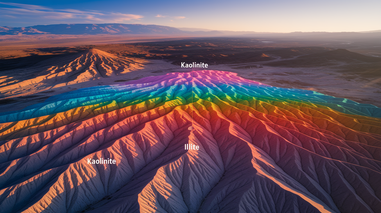
Hyperion, aboard NASA’s EO-1, showed early orbital hyperspectral mineral mapping by imaging hydrothermal alteration zones in Nevada’s Great Basin. Analysts used continuum removal to isolate features near 2.2 µm and mapped spatial patterns of kaolinite, alunite, and illite that lined up with known epithermal gold deposits. The work proved that orbital hyperspectral data could map alteration minerals at reconnaissance scale, shrinking the area needing ground follow up and steering field campaigns to the best zones.
WorldView-3, a commercial satellite with eight SWIR bands, has been used to map carbonate formations in arid regions. WorldView-3 isn’t a true hyperspectral sensor, but its SWIR bands bracket the 2.3 µm carbonate absorption. Band ratios and spectral indices from those bands successfully separated calcite rich from dolomite rich units in exposed desert outcrops in North Africa. WorldView-3’s spatial resolution (better than 4 meters in multispectral mode) let geologists tie spectral units to stratigraphic boundaries visible in high resolution imagery, tightening geologic mapping accuracy.
AVIRIS-NG, an airborne hyperspectral sensor, flew over clay rich badlands in the western U.S. to classify clay mineral assemblages tied to paleoclimate shifts. The sensor’s 5 nanometer sampling across the SWIR resolved subtle shifts in the 2.2 µm absorption, letting researchers map gradients from smectite dominated zones (wetter paleoclimates) to illite dominated zones (drier conditions). The resulting mineral maps were checked against X ray diffraction of field samples and showed close agreement, proving the precision you can get with quality hyperspectral data and solid atmospheric correction.
Limitations and Sources of Error
Mixed pixels are the biggest headache in orbital mineral mapping. A 30 meter pixel from a multispectral sensor or even a 10 meter pixel from a hyperspectral sensor often holds multiple minerals, vegetation, soil, and rock fragments. The observed spectrum is a blend, and pulling out the contribution of a minor phase requires spectral unmixing and high signal to noise. If the target mineral covers less than about 5 to 10 percent of the pixel and its spectral contrast with background is weak, detection gets unreliable.
Atmospheric contamination lingers even after correction. Water vapor variability, undetected thin clouds, and aerosol plumes leave residual errors in surface reflectance. Bands near 1.4 µm and 1.9 µm are often unusable because atmospheric water vapor absorption is so strong that small correction errors blow up into large reflectance errors. Sensor noise, especially in the SWIR where detectors are noisier than in visible, cuts the ability to catch shallow absorption features. Some minerals, like certain sulfates and phyllosilicates, have very similar SWIR spectra. Telling them apart needs either extra wavelength coverage (thermal infrared) or independent geochemical data. Topographic shadowing, surface roughness, and variable illumination add another layer, requiring correction algorithms that account for slope, aspect, and local shading.
Final Words
In the action, orbital sensors catch sunlight off the ground and turn that light into reflectance curves. Those curves show absorption features tied to mineral bonds, so we can separate clays, carbonates, and iron oxides.
Hyperspectral and multispectral sensors cover VNIR, SWIR, and thermal infrared. After atmospheric and radiometric correction we match spectra to libraries and run algorithms, but mixed pixels and surface cover can still confuse results.
This piece focused on using spectral signatures to distinguish minerals from orbital sensors and the practical workflow. With the right sensor and careful processing, orbital mineral mapping points you to good places for follow up.
FAQ
Q: What is the spectral signature of a mineral?
A: The spectral signature of a mineral is its pattern of reflected or emitted light across wavelengths, showing absorption and reflectance features tied to chemistry and structure, like a fingerprint used to tell minerals apart in lab or from orbit.
Q: What are the 8 ways to identify minerals?
A: The eight common ways to identify minerals are color, streak, luster, hardness, cleavage or fracture, specific gravity, magnetism, and acid reaction; combine tests because single traits can mislead.
Q: What is the most reliable way to identify a mineral using color?
A: The most reliable way to identify a mineral using color is to check its streak (the powdered color) and compare to references, since surface color often changes with impurities or weathering.
Q: Why are spectral signatures important?
A: Spectral signatures are important because they reveal mineral chemistry and bonding through diagnostic absorption bands, letting scientists map compositions from orbit and infer geological processes.